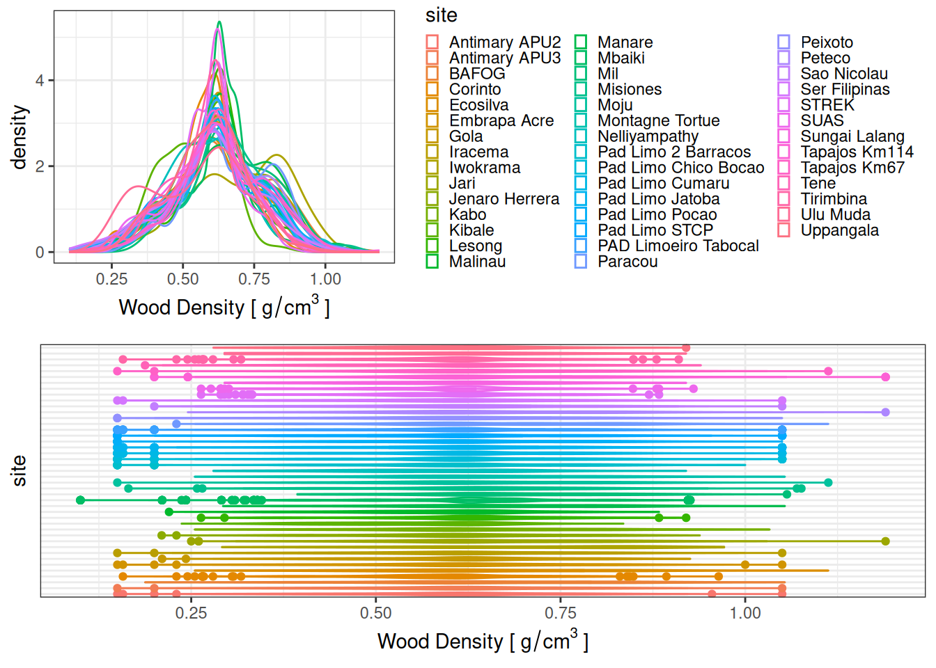
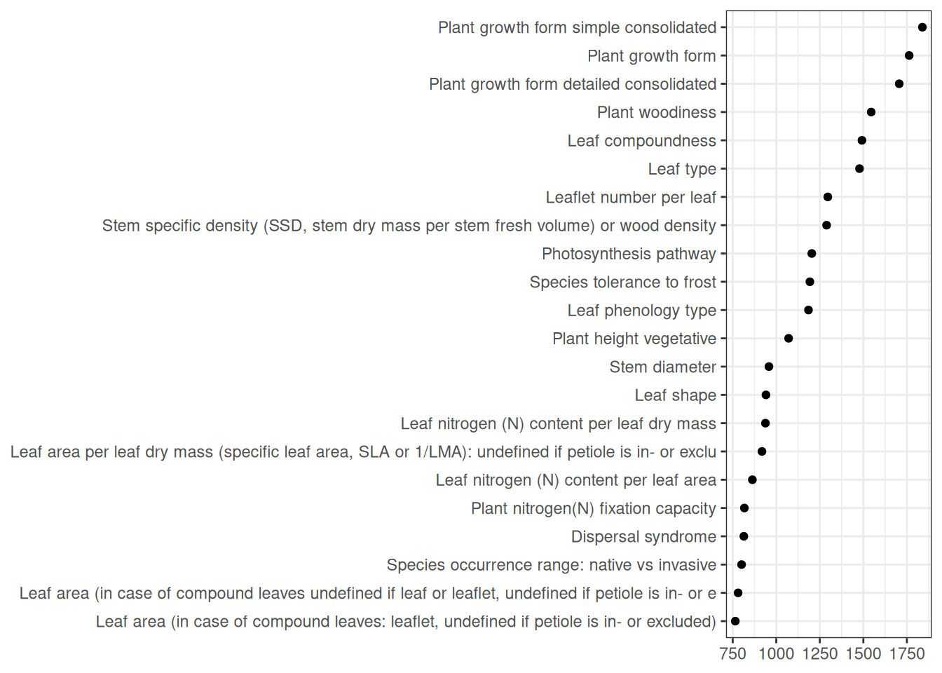
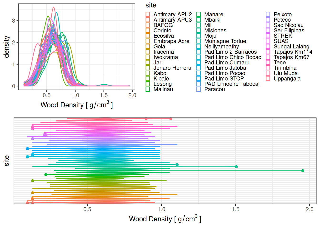
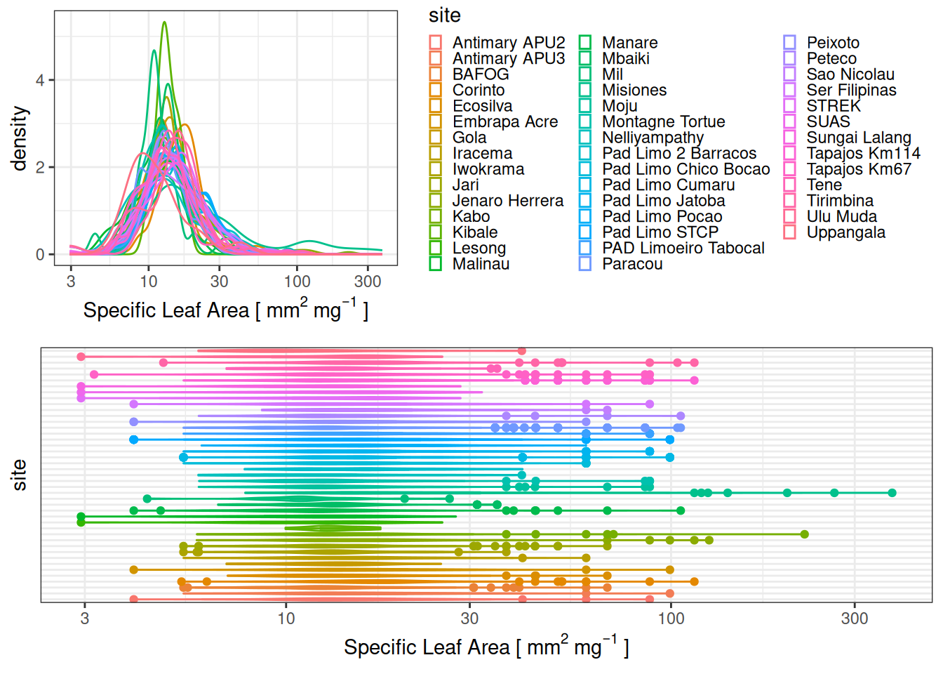
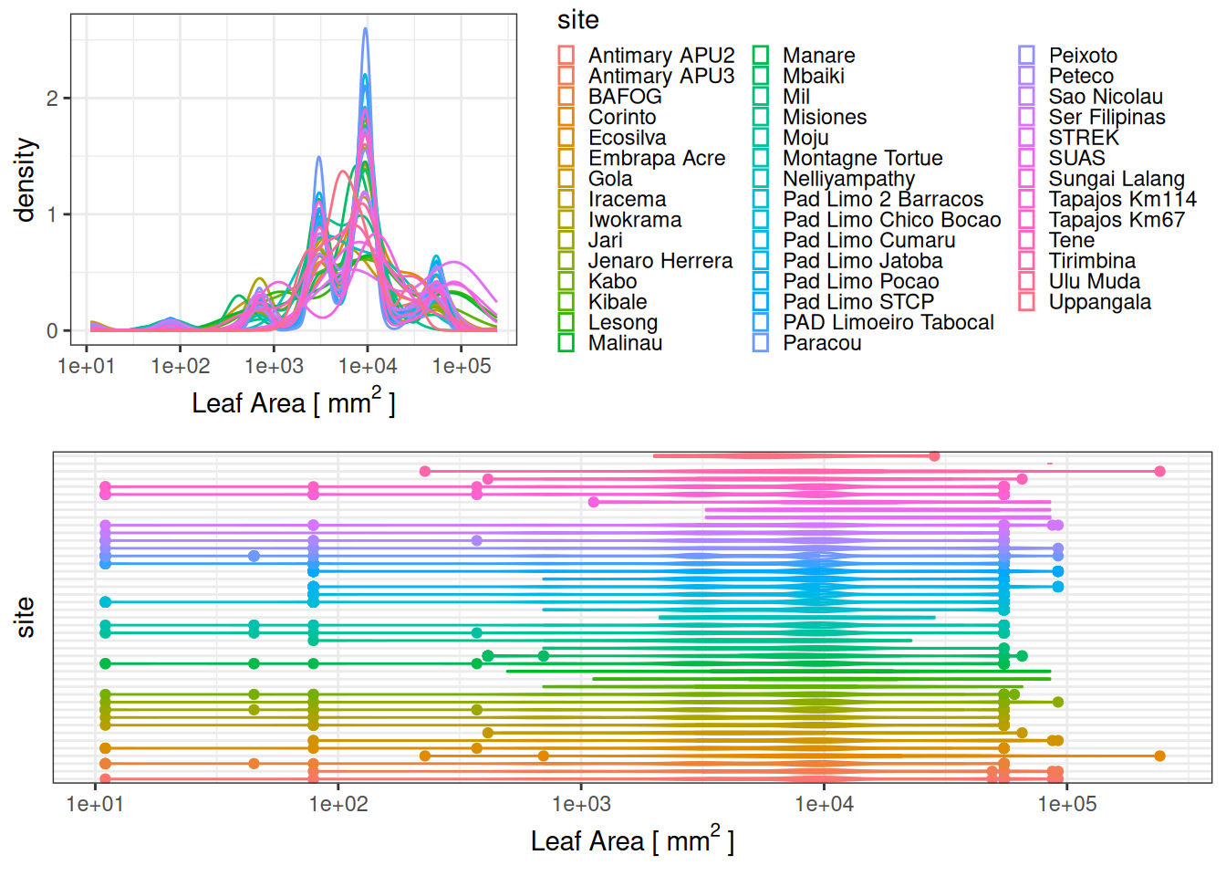
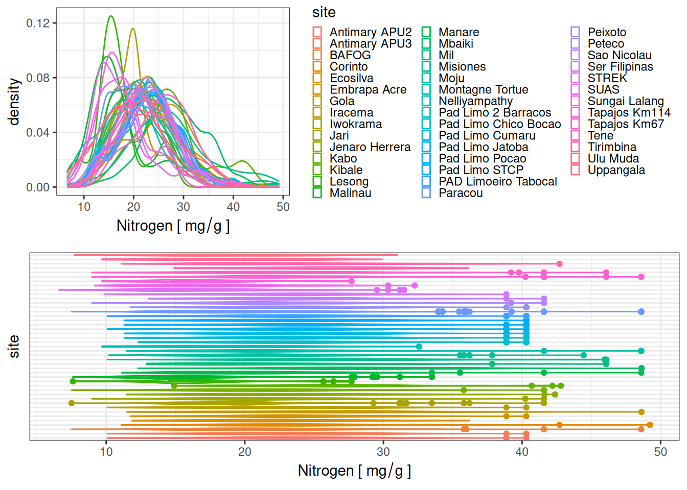
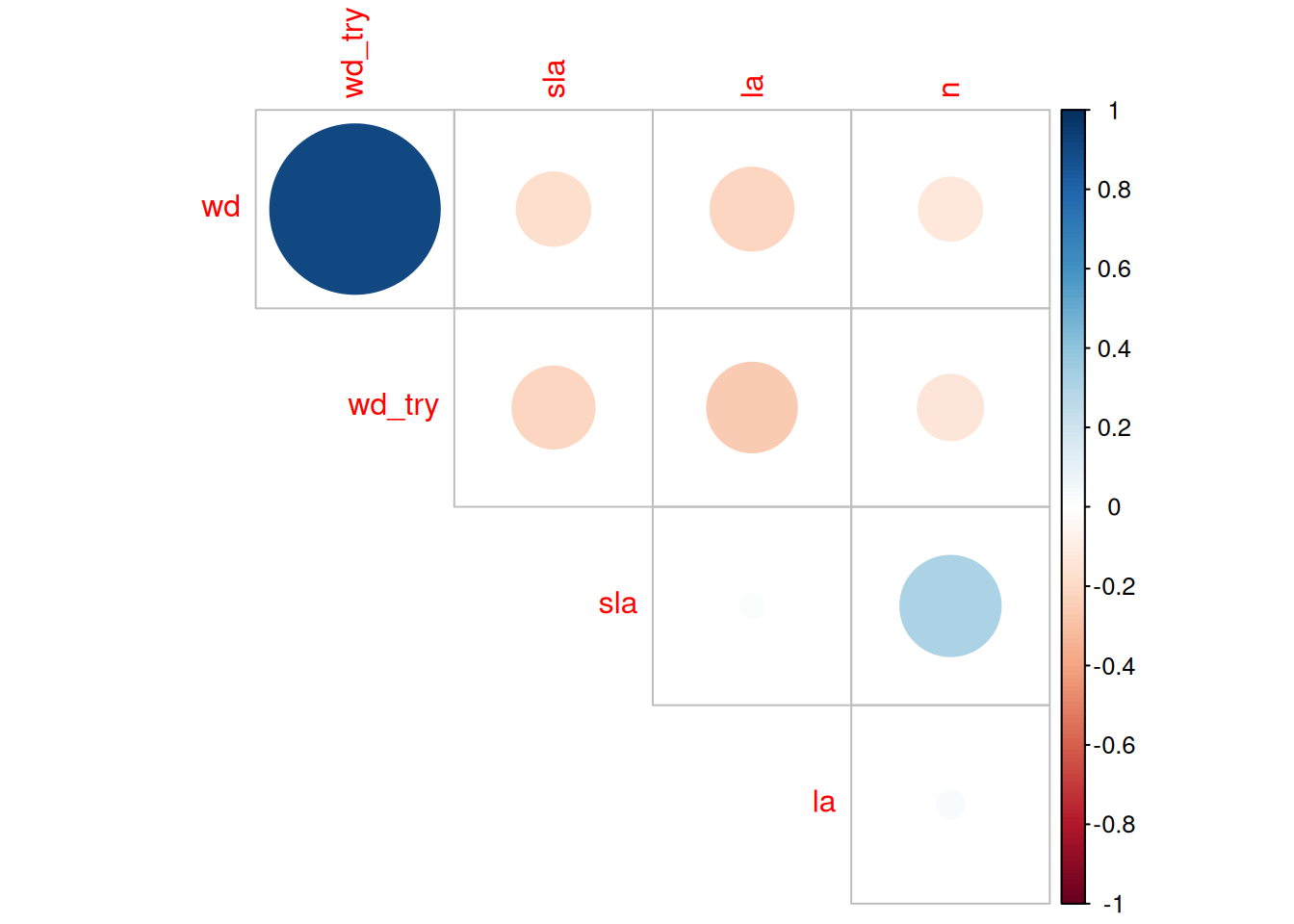
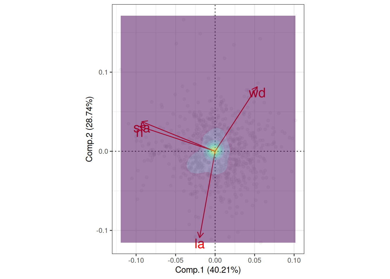
Functional

We used cleaned taxonomy to retrieve data from TRY (Kattge et al. 2019) and BIOMASS (Réjou-Méchain et al. 2017). This corresponds to version 6.

Wood density

Using BIOMASS (Réjou-Méchain et al. 2017), we retrieved wood density for most species, with little differences between sites means.

Code

taxo <- read_tsv(taxonomy_file)
wd <- getWoodDensity(taxo$genus_cleaned, taxo$species_cleaned) %>%
  group_by(genus, species) %>%
  summarise(wd = mean(meanWD)) %>%
  na.omit() %>%
  rename(genus_cleaned = genus, species_cleaned = species)
taxo_wd <- left_join(taxo, wd)
g1 <- ggplot(taxo_wd, aes(wd, col = site)) +
  geom_density() +
  theme_bw() +
  xlab(expression("Wood Density [" ~ g / cm^3 ~ "]")) +
  theme(legend.key.size = unit(.5, "line"))
g2 <- ggplot(taxo_wd, aes(site, wd, col = site)) +
  geom_violin() +
  geom_boxplot(width = .2) +
  coord_flip() +
  theme_bw() +
  theme(
    legend.position = "none",
    axis.text.y = element_blank(),
    axis.ticks.y = element_blank()
  ) +
  ylab(expression("Wood Density [" ~ g / cm^3 ~ "]"))
cowplot::plot_grid(g1, g2, nrow = 2)

Wood density extracted from Réjou-Méchain et al. (2017).

TRY

In order to make a request for data on TRY (Kattge et al. 2019), we first retrieved the total species list available from TRY and matched our species to their species list to obtain corresponding species ID on TRY. By chance TRY is also using WordFlora reference. But they limit the requests to 200 species. We thus retrieved available species data by batch of 200 (see example below).

Code

try_sp <- read_tsv(taxonomy_file) %>%
  select(scientific_cleaned) %>%
  na.omit() %>%
  unique() %>%
  left_join(read_tsv("data/raw_data/TryAccSpecies.txt"),
    by = c("scientific_cleaned" = "AccSpeciesName")
  )
sp_req <- try_sp %>%
  select(AccSpeciesID) %>%
  na.omit() %>%
  unique() %>%
  arrange() %>%
  mutate(request = rep(1:100, each = 200)[seq_len(n())]) %>%
  group_by(request) %>%
  summarise(species_list = paste0(AccSpeciesID, collapse = ", "))
write_tsv(sp_req, "data/derived_data/try_species_requests.tsv")

Code

read_tsv("data/derived_data/try_species_requests.tsv", n_max = 1) %>%
  kable(caption = "Example of species ID list for TRY Data Explorer requests (limited to 200) for the first chunk.") # nolint

Example of species ID list for TRY Data Explorer requests (limited to 200) for the first chunk.

request

species_list

1

53035, 8582, 14866, 53654, 14156, 15557, 27269, 56630, 29126, 52505, 31260, 30552, 4136, 17195, 8580, 32629, 39236, 8980, 3147, 86888, 52969, 38544, 30609, 27124, 36681, 39724, 26812, 40311, 36684, 37540, 46572, 34387, 44223, 22256, 49908, 52432, 13692, 430788, 33337, 44232, 5583, 30895, 12681, 43766, 54284, 30632, 33380, 52899, 246054, 56788, 12678, 43849, 11219, 14450, 18719, 14882, 56617, 33288, 24884, 38616, 34870, 20736, 408207, 50321, 54536, 54783, 103114, 40645, 35216, 30904, 44986, 25648, 52844, 40368, 41051, 22281, 32634, 430797, 30624, 52895, 44853, 37333, 43959, 43542, 33334, 21888, 26519, 38552, 45280, 29808, 20479, 15619, 40831, 19480, 55518, 47684, 19696, 55524, 36897, 44855, 55866, 56813, 52968, 92496, 43763, 4160, 7610, 10273, 17778, 40357, 11353, 56697, 27177, 57266, 38516, 53047, 29162, 22272, 50499, 46274, 54663, 43873, 57627, 57282, 52436, 30575, 14860, 43767, 39875, 32613, 14890, 21873, 99866, 29834, 74946, 5605, 52900, 12272, 33343, 27264, 8569, 39234, 42597, 84130, 10716, 40823, 40360, 11365, 40231, 11345, 44590, 43958, 37888, 8576, 18800, 101052, 53039, 35441, 32627, 3383, 50390, 39604, 29655, 57424, 56781, 35358, 55852, 35649, 54098, 11952, 3878, 34856, 51769, 36686, 38676, 38574, 3877, 50523, 33335, 5937, 6614, 19578, 22258, 52390, 3446, 51785, 22261, 38551, 43836, 33295, 43828, 13282, 32615, 50507, 54280, 29811, 43810, 19522, 30614, 2458

Next we could investigate trait data available for more than 40% of species, which were not many.

Code

list.files("data/derived_data/try_req/", full.names = TRUE) %>%
  lapply(read_tsv, skip = 3) %>%
  lapply(gather, species, N, -Trait, -TraitID) %>%
  bind_rows() %>%
  filter(N > 0) %>%
  group_by(Trait, TraitID) %>%
  summarise(N = n()) %>%
  filter(N > 0.4 * 1901) %>%
  ggplot(aes(fct_rev(fct_infreq(Trait, N)), N)) +
  geom_point() +
  theme_bw() +
  coord_flip() +
  theme(axis.title = element_blank())

Traits available for at least 50% of species available on TRY.

For the first test we thus used:

• 14: Leaf nitrogen (N) content per leaf dry mass, mg/g
• 3117: Leaf area per leaf dry mass (specific leaf area, SLA or 1/LMA): undefined if petiole is in- or excluded, mm2 mg-1
• 4: Stem specific density (SSD, stem dry mass per stem fresh volume) or wood density, g/cm3
• 3114: Leaf area (in case of compound leaves: leaflet, undefined if petiole is in- or excluded), mm2

The request takes times to be ready. Moreover, we should try to minimise the number of requests. This was a first test. But future tests should be discussed before.

Code

taxo <- read_tsv(taxonomy_file)
traits <- c(
  "Stem specific density (SSD, stem dry mass per stem fresh volume) or wood density", # nolint
  "Leaf area per leaf dry mass (specific leaf area, SLA or 1/LMA): undefined if petiole is in- or excluded", # nolint
  "Leaf nitrogen (N) content per leaf dry mass",
  "Leaf area (in case of compound leaves undefined if leaf or leaflet, undefined if petiole is in- or excluded)" # nolint
)
try <- read_tsv("data/raw_data/try/38775.txt") %>%
  filter(TraitName %in% traits) %>%
  filter(AccSpeciesName %in% taxo$scientific_cleaned) %>%
  select(AccSpeciesName, TraitName, StdValue) %>%
  rename(
    species = AccSpeciesName,
    trait = TraitName,
    value = StdValue
  ) %>%
  mutate(trait = recode(trait,
    "Stem specific density (SSD, stem dry mass per stem fresh volume) or wood density" = "wd", # nolint
    "Leaf area per leaf dry mass (specific leaf area, SLA or 1/LMA): undefined if petiole is in- or excluded" = "sla", # nolint
    "Leaf nitrogen (N) content per leaf dry mass" = "n",
    "Leaf area (in case of compound leaves undefined if leaf or leaflet, undefined if petiole is in- or excluded)" = "la" # nolint
  )) %>%
  group_by(species, trait) %>%
  summarise(value = mean(as.numeric(value), na.rm = TRUE)) %>%
  pivot_wider(values_from = "value", names_from = "trait")
write_tsv(try, "data/derived_data/try_extract.tsv")

Code

try <- read_tsv("data/derived_data/try_extract.tsv") %>%
  rename(scientific_cleaned = species) %>%
  rename(wd_try = wd)
taxo <- read_tsv(taxonomy_file)
taxo_try <- left_join(taxo, try)

We obtained numerous data across species for SLA, WD, and N:

Code

g1 <- ggplot(taxo_try, aes(wd_try, col = site)) +
  geom_density() +
  theme_bw() +
  xlab(expression("Wood Density [" ~ g / cm^3 ~ "]")) +
  theme(legend.key.size = unit(.5, "line"))
g2 <- ggplot(taxo_try, aes(site, wd_try, col = site)) +
  geom_violin() +
  geom_boxplot(width = .2) +
  coord_flip() +
  theme_bw() +
  theme(
    legend.position = "none",
    axis.text.y = element_blank(),
    axis.ticks.y = element_blank()
  ) +
  ylab(expression("Wood Density [" ~ g / cm^3 ~ "]"))
cowplot::plot_grid(g1, g2, nrow = 2)

Wood density extracted from Kattge et al. (2019).

Code

g1 <- ggplot(taxo_try, aes(sla, col = site)) +
  geom_density() +
  theme_bw() +
  xlab(expression("Specific Leaf Area [" ~ mm^2 ~ mg^{
    -1
  } ~ "]")) +
  scale_x_log10() +
  theme(legend.key.size = unit(.5, "line"))
g2 <- ggplot(taxo_try, aes(site, sla, col = site)) +
  geom_violin() +
  geom_boxplot(width = .2) +
  coord_flip() +
  theme_bw() +
  theme(
    legend.position = "none",
    axis.text.y = element_blank(),
    axis.ticks.y = element_blank()
  ) +
  ylab(expression("Specific Leaf Area [" ~ mm^2 ~ mg^{
    -1
  } ~ "]")) +
  scale_y_log10()
cowplot::plot_grid(g1, g2, nrow = 2)

Specific leaf area extracted from Kattge et al. (2019).

Code

g1 <- ggplot(taxo_try, aes(la, col = site)) +
  geom_density() +
  theme_bw() +
  xlab(expression("Leaf Area [" ~ mm^2 ~ "]")) +
  scale_x_log10() +
  theme(legend.key.size = unit(.5, "line"))
g2 <- ggplot(taxo_try, aes(site, la, col = site)) +
  geom_violin() +
  geom_boxplot(width = .2) +
  coord_flip() +
  theme_bw() +
  theme(
    legend.position = "none",
    axis.text.y = element_blank(),
    axis.ticks.y = element_blank()
  ) +
  ylab(expression("Leaf Area [" ~ mm^2 ~ "]")) +
  scale_y_log10()
cowplot::plot_grid(g1, g2, nrow = 2)

Leaf area extracted from Kattge et al. (2019).

Code

g1 <- ggplot(taxo_try, aes(n, col = site)) +
  geom_density() +
  theme_bw() +
  xlab(expression("Nitrogen [" ~ mg / g ~ "]")) +
  theme(legend.key.size = unit(.5, "line"))
g2 <- ggplot(taxo_try, aes(site, n, col = site)) +
  geom_violin() +
  geom_boxplot(width = .2) +
  coord_flip() +
  theme_bw() +
  theme(
    legend.position = "none",
    axis.text.y = element_blank(),
    axis.ticks.y = element_blank()
  ) +
  ylab(expression("Nitrogen [" ~ mg / g ~ "]"))
cowplot::plot_grid(g1, g2, nrow = 2)

Leaf nitrogen extracted from Kattge et al. (2019).

All raw

We assembled all traits data from TRY (Kattge et al. 2019), BIOMASS (Réjou-Méchain et al. 2017), and TALLO (Jucker et al. 2022), and obtained the following correlations:

Code

taxo_traits <- taxo %>%
  left_join(wd) %>%
  left_join(try)

Code

taxo_traits %>%
  select(site, scientific_cleaned, wd, la, sla, n, wd_try) %>%
  gather(trait, value, -site, -scientific_cleaned) %>%
  na.omit() %>%
  group_by(site, trait, scientific_cleaned) %>%
  summarise(mean = mean(value)) %>%
  group_by(site, trait) %>%
  summarise(n = n()) %>%
  pivot_wider(names_from = trait, values_from = n) %>%
  kable()

site	la	n	sla	wd	wd_try
Antimary APU2	131	125	118	161	129
Antimary APU3	108	102	100	139	110
BAFOG	224	230	232	311	244
Corinto	163	175	196	262	174
Ecosilva	122	112	106	160	122
Embrapa Acre	122	118	113	158	121
Gola	20	68	31	240	132
Iracema	159	142	133	200	156
Iwokrama	90	73	73	113	93
Jari	282	237	219	390	270
Jenaro Herrera	230	182	169	331	191
Kabo	181	153	158	240	184
Kibale	7	26	12	75	43
Lesong	4	21	25	76	57
Malinau	15	101	146	497	316
Manare	153	181	187	226	150
Mbaiki	20	93	34	369	169
Mil	40	29	21	48	34
Misiones	24	38	57	115	74
Moju	258	217	200	325	247
Montagne Tortue	181	202	212	249	177
Nelliyampathy	6	12	11	69	38
PAD Limoeiro Tabocal	150	140	132	189	146
Pad Limo 2 Barracos	84	75	70	103	81
Pad Limo Chico Bocao	133	125	119	166	133
Pad Limo Cumaru	146	132	126	183	144
Pad Limo Jatoba	135	123	118	166	136
Pad Limo Pocao	91	84	81	114	88
Pad Limo STCP	130	121	116	158	127
Paracou	352	370	382	538	358
Peixoto	127	117	111	174	123
Peteco	221	199	187	295	210
STREK	9	76	111	314	211
SUAS	10	52	75	194	125
Sao Nicolau	95	90	82	117	96
Ser Filipinas	99	99	92	132	102
Sungai Lalang	3	18	23	68	50
Tapajos Km114	286	252	224	373	264
Tapajos Km67	259	232	210	367	252
Tene	25	59	36	196	105
Tirimbina	185	199	218	291	195
Ulu Muda	1	13	14	43	30
Uppangala	9	21	19	121	78

Code

taxo_traits %>%
  select(wd, wd_try, sla, la, n) %>%
  cor(use = "pairwise.complete.obs") %>%
  corrplot::corrplot(type = "upper", diag = FALSE)

All imputed

We used missing data imputation with random forest for with the missForest R package to further impute missing trait values (Gendre et al. 2024). We first aggregated data at the genus level with median trait value to inform genus lacking traits data or species. We obtained for imputation a normalised root mean square error of NRMSE=1.007. We obtained the global PCA below showed globally and per site.

Code

raw <- taxo_traits %>%
  filter(!is.na(genus_cleaned)) %>%
  select(genus_cleaned, wd, sla, la, n) %>%
  group_by(genus_cleaned) %>%
  summarise_all(median, na.rm = TRUE) %>%
  filter(!(is.na(wd) & is.na(sla) & is.na(la) & is.na(n)))
imputation <- missForest::missForest(
  raw %>%
    select(-genus_cleaned) %>%
    as.data.frame(),
  verbose = TRUE
)
imputation$OOBerror
imputation$ximp %>%
  mutate(genus_cleaned = raw$genus_cleaned, .before = 1) %>%
  write_tsv("data/derived_data/imputed_traits.tsv")

Code

imputed <- read_tsv("data/derived_data/imputed_traits.tsv")
autoplot(
  princomp(select(imputed, wd, sla, la, n) %>%
    mutate(sla = log(sla), la = log(la)), cor = TRUE),
  data = imputed, alpha = 0.25, col = "lightgrey",
  loadings.label.size = 6,
  loadings.label.colour = "red", loadings.label.vjust = 1.1,
  loadings.label.repel = TRUE,
  loadings = TRUE, loadings.label = TRUE, loadings.colour = "red"
) +
  coord_equal() +
  geom_hline(aes(yintercept = 0), col = "black", linetype = "dotted") +
  geom_vline(aes(xintercept = 0), col = "black", linetype = "dotted") +
  theme_bw() +
  geom_density_2d_filled(alpha = .5) +
  theme(legend.position = "none")

Imputed traits global principal component analysis.

Traits data

All traits data are saved in outputs/traits_vX.tsv with the following columns:

• scientific_cleaned: the cleaned scientific name for junction with the taxonomic data
• trait: the trait acronym or code
• species_trait_value_raw: the species median trait raw value from TRY
• genus_trait_value_imputed: the genus median trait imputed value in case of missing raw values
• definition: the trait definition
• unit: the trait unit

Code

all_traits <- taxo_traits %>%
  select(scientific_cleaned, genus_cleaned, wd, sla, la, n) %>%
  gather(
    trait, species_trait_value_raw,
    -scientific_cleaned, -genus_cleaned
  ) %>%
  filter(!is.na(scientific_cleaned)) %>%
  unique() %>%
  left_join(imputed %>%
    select(genus_cleaned, wd, sla, la, n) %>%
    gather(trait, genus_trait_value_imputed, -genus_cleaned)) %>%
  mutate(trait = recode(trait,
    "wd" = "WD", "sla" = "SLA",
    "la" = "LA", "n" = "N"
  )) %>%
  mutate(definition = recode(trait,
    "WD" = "Stem specific wood density",
    "SLA" = "Specific leaf area",
    "LA" = "Leaf area",
    "N" = "Leaf nitrogen content per leaf dry mass",
    "hmax" = "Asymptotic height"
  )) %>%
  mutate(unit = recode(trait,
    "WD" = "g cm-3",
    "SLA" = "mm2 mg-1",
    "LA" = "mm2",
    "N" = "mg g-1",
    "hmax" = "m"
  ))
write_tsv(all_traits, traits_file)

Code

traits <- read_tsv(traits_file)
taxo <- read_tsv(taxonomy_file)
taxo %>%
  filter(
    !is.na(scientific_cleaned),
    !is.na(species_cleaned)
  ) %>%
  select(scientific_cleaned) %>%
  unique() %>%
  mutate(trait = scientific_cleaned %in% traits$scientific_cleaned) %>%
  filter(!trait)

Gendre, Matthieu, Torsten Hauffe, Catalina Pimiento, and Daniele Silvestro. 2024. “Benchmarking Imputation Methods for Categorical Biological Data.” Methods in Ecology and Evolution 15 (9): 1624–38.

Jucker, Tommaso, Fabian Jörg Fischer, Jérôme Chave, David A. Coomes, John Caspersen, Arshad Ali, Grace Jopaul Loubota Panzou, et al. 2022. “Tallo: A Global Tree Allometry and Crown Architecture Database.” Global Change Biology 28 (17): 5254–68. https://doi.org/10.1111/gcb.16302.

Kattge, Jens, Gerhard Bönisch, Sandra Díaz, Sandra Lavorel, Iain Colin Prentice, Paul Leadley, Susanne Tautenhahn, et al. 2019. “TRY Plant Trait Database Enhanced Coverage and Open Access.” Global Change Biology 26 (1): 119–88. https://doi.org/10.1111/gcb.14904.

Réjou-Méchain, Maxime, Ariane Tanguy, Camille Piponiot, Jérôme Chave, and Bruno Hérault. 2017. “Biomass: An r Package for Estimating Above-Ground Biomass and Its Uncertainty in Tropical Forests.” Edited by Sarah Goslee. Methods in Ecology and Evolution 8 (9): 1163–67. https://doi.org/10.1111/2041-210x.12753.