Joint Genus

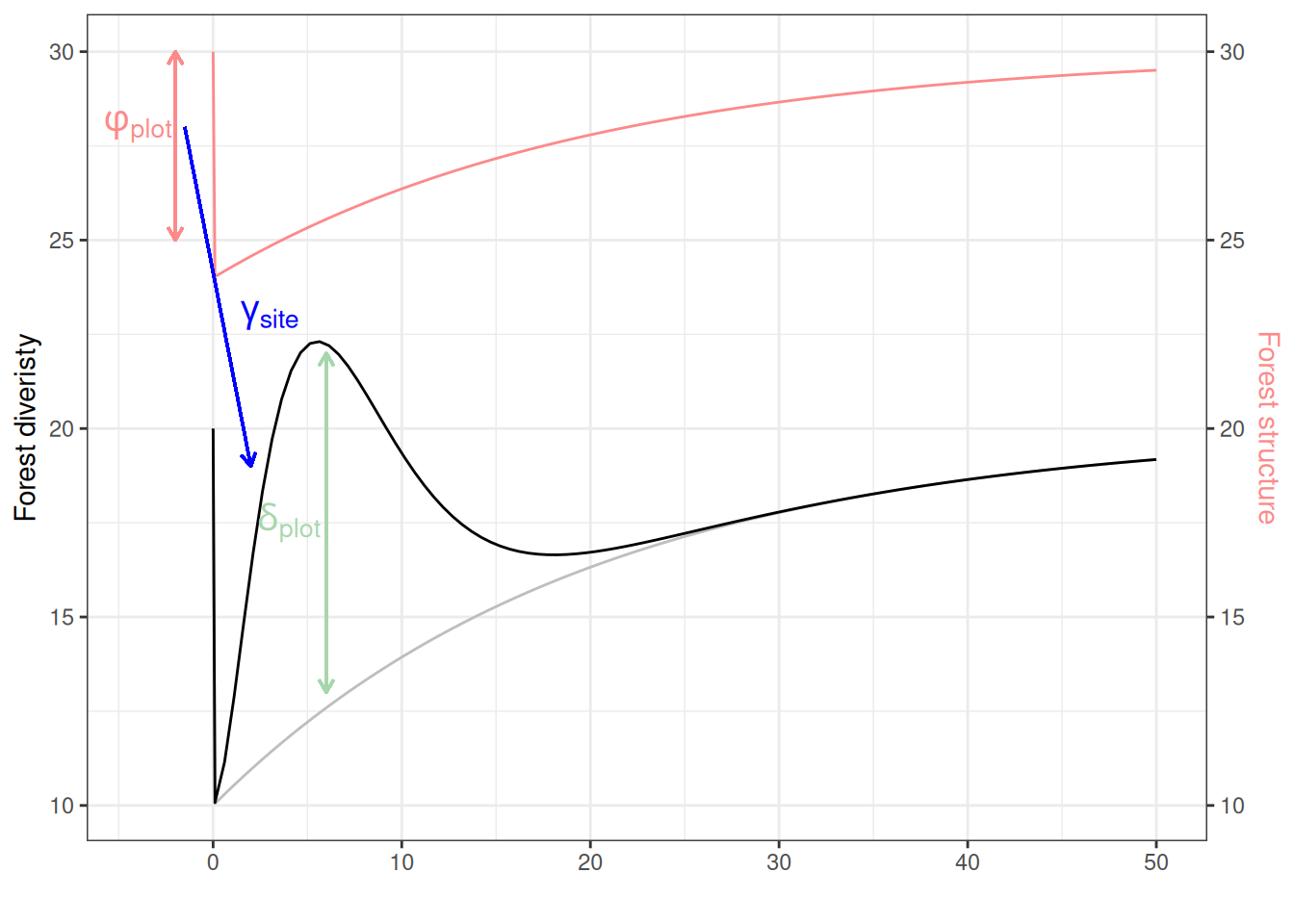
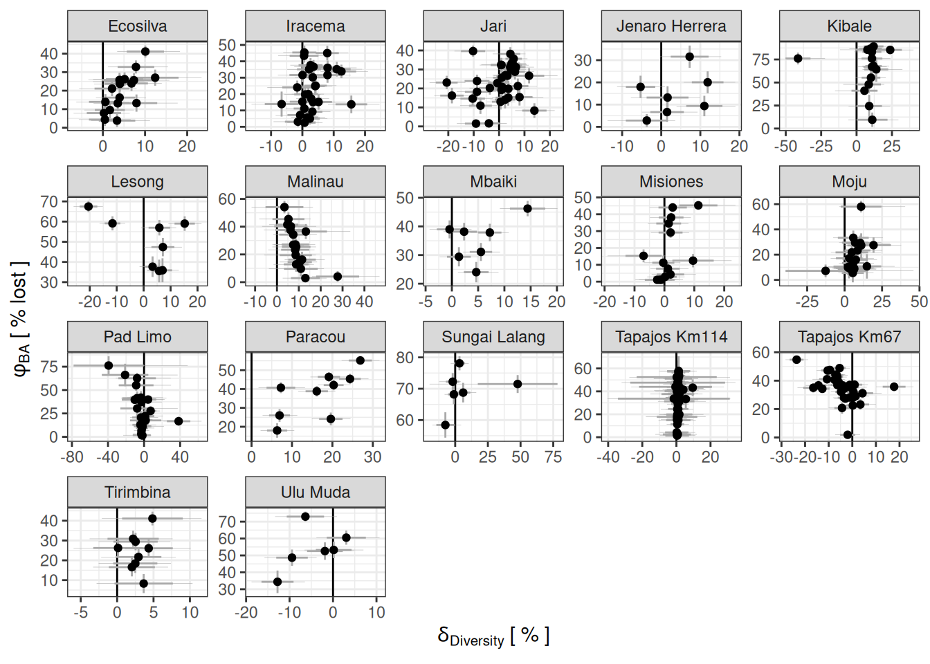
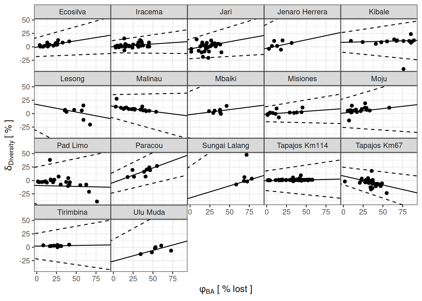
The model is the same as the modelling framework, but we want to establish a connection between the trajectory of forest structure, as represented by basal area, and forest diversity, as represented by genus diversity.

Equilibirum

Equilibrium model using control and pre-logging inventories to inform \(\theta\) prior of the recovery trajectory:

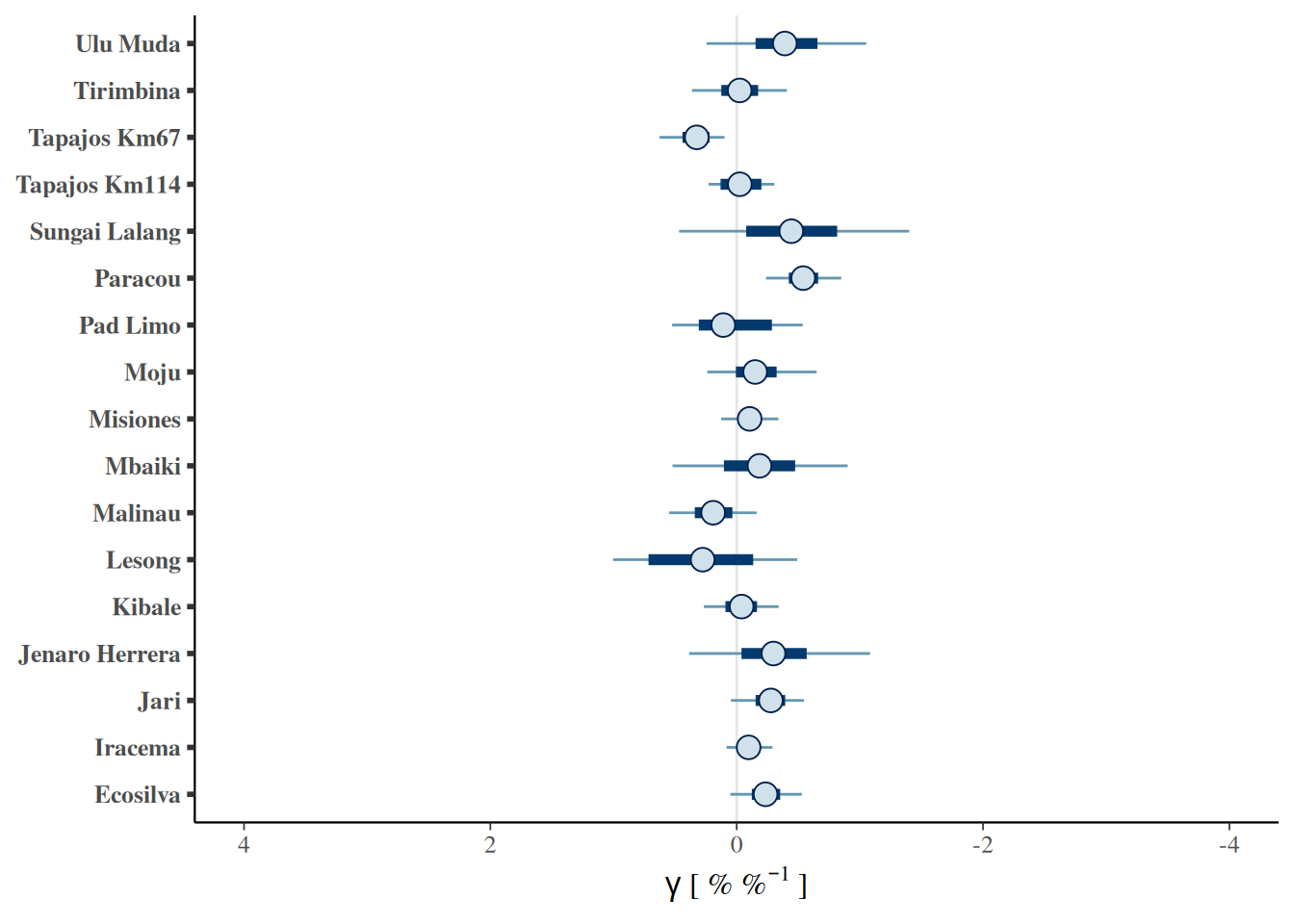
\[ \begin{align} BA \sim \mathcal N (\mu_{BA,site}+\delta_{BA,plot}, \sigma_{BA})\\ \delta_{BA,plot} \sim \mathcal N(0,\sigma_{BA,plot}) \\ y \sim \mathcal N (\mu_{site}+\delta_{plot}, \sigma)\\ \delta_{plot} \sim \mathcal N(0,\sigma_{plot}) \end{align} \]

Recovery

Recovery trajectory model:

\[ \begin{align} log(BA) \sim \mathcal N (log(\mu_{BA}), \sigma_{BA})\\ \mu_{BA} = \theta_{BA,site} \times (\phi_{BA,plot} + LTP_{BA} \times (1 - \phi_{plot}) + STP_{BA}) \\ LTP_{BA} = 1 - e^{-\lambda_{BA,plot} \times t} \\ STP_{BA} = \delta_{BA,plot} \times (\frac{t}{\tau_{BA,site}} \times e^{1-\frac{t}{\tau_{BA,site}}})^2 \\ log(y) \sim \mathcal N (log(\mu), \sigma)\\ \mu = \theta_{site} \times (\phi_{plot} + LTP \times (1 - \phi_{plot}) + STP) \\ LTP = 1 - e^{-\lambda_{plot} \times t} \\ STP = \delta_{plot} \times (\frac{t}{\tau_{site}} \times e^{1-\frac{t}{\tau_{site}}})^2 \\ \delta_{plot} \sim \mathcal N ( \delta0_{site}+\phi_{BA,plot} \times \gamma_{site}, \sigma_{\delta}) \end{align} \]

With the big novelty being:

\[ \delta_{plot} \sim \mathcal N ( \delta0_{site}+\phi_{BA,plot} \times \gamma_{site}, \sigma_{\delta}) \]

With the function linking the two to be defined.

Code

ltp <- function(time, dist, thetainf, lambda) {
  theta0 <- thetainf * dist
  ltp <- 1 - exp(-lambda * time)
  theta0 + (thetainf - theta0) * (ltp)
}
stp <- function(time, dist, thetainf, lambda, tau, delta) {
  theta0 <- thetainf * dist
  ltp <- 1 - exp(-lambda * time)
  stp <- delta * (time / tau * exp(1 - time / tau))^2
  theta0 + ltp * (thetainf - theta0) + stp * thetainf
}
data.frame(time = seq(0.1, 50, length.out = 100)) %>%
  mutate(y_ba = stp(time,
    dist = 0.8, thetainf = 30, lambda = 0.05,
    tau = 5, delta = 0
  )) %>% 
  mutate(y_stp = stp(time,
    dist = 0.5, thetainf = 20, lambda = 0.05,
    tau = 5, delta = 0.5
  )) %>%
  mutate(y_ltp = ltp(time, dist = 0.5, thetainf = 20, lambda = 0.05)) %>%
  bind_rows(data.frame(time = 0, y_stp = 20, y_ltp = 20, y_ba = 30)) %>%
  ggplot(aes(time)) +
  geom_line(aes(y = y_ba), col = "#fc8a8a") +
  geom_line(aes(y = y_ltp), col = "grey") +
  geom_line(aes(y = y_stp)) +
  theme_bw() +
  xlab("") + 
  scale_y_continuous(
    name = "Forest diveristy",
    sec.axis = sec_axis(~.*1, name = "Forest structure")
  ) +
  theme(
    axis.title.y.right = element_text(color = "#fc8a8a")
  ) +
  annotate("text",
    x = -4, y = 28, label = "phi[plot]",
    col = "#fc8a8a", parse = TRUE, size = 5
  ) +
    geom_segment(aes(x = -2, y = 25, xend = -2, yend = 30),
    arrow = arrow(length = unit(0.2, "cm")), col = "#fc8a8a"
  ) +
  geom_segment(aes(x = -2, y = 30, xend = -2, yend = 25),
    arrow = arrow(length = unit(0.2, "cm")), col = "#fc8a8a"
  ) +
  annotate("text",
    x = 4, y = 17.5, label = "delta[plot]",
    col = "#a7d6ac", parse = TRUE, size = 5
  ) +
  geom_segment(aes(x = 6, y = 13, xend = 6, yend = 22),
    arrow = arrow(length = unit(0.2, "cm")), col = "#a7d6ac"
  ) +
  geom_segment(aes(x = 6, y = 22, xend = 6, yend = 13),
    arrow = arrow(length = unit(0.2, "cm")), col = "#a7d6ac"
  ) +
  geom_segment(aes(x = -1.5, y = 28, xend = 2, yend = 19),
    arrow = arrow(length = unit(0.2, "cm")), col = "blue"
  ) +
  annotate("text",
    x = 3, y = 23, label = "gamma[site]",
    col = "blue", parse = TRUE, size = 5
  )

STP proj with pars.

Code

recovery <- cmdstan_model("models/recovery.stan")
data <- read_tsv("../modelling/data/derived_data/data_rec.tsv", col_types = cols()) %>%
    select(-y) %>% 
    filter(variable %in% c("ba", "diversity_q1_gen")) %>%
    select(-sitenum, -plotnum) %>% 
    pivot_wider(names_from = variable, values_from = value) %>% 
    na.omit() %>% 
    filter(!(site %in% c("Manare", "Montagne Tortue", "Nelliyampathy",
                         "Uppangala", "BAFOG", "Sao Nicolau",
                         "Kabo", "Mil", "Corinto",
                         "Peixoto", "Iwokrama", "Antimary", "Peteco"))) %>% 
    mutate(sitenum = as.numeric(as.factor(site))) %>% 
    mutate(plotnum = as.numeric(as.factor(paste(site, plot)))) %>% 
    arrange(sitenum, plotnum, rel_year)
ind <- data %>%
    select(site, plot, sitenum, plotnum) %>%
    unique()
ba_priors <- read_tsv(file.path("..", "modelling",
                                "chains", paste0("equ_", "ba"), "mu.tsv")) %>% 
    select(-sitenum) %>% 
    left_join(select(ind, site, sitenum) %>% unique()) %>% 
    na.omit()
div_priors <- read_tsv(file.path("..", "modelling",
                                 "chains", paste0("equ_", "diversity_q1_gen"),
                                 "mu.tsv")) %>% 
    select(-sitenum) %>% 
    left_join(select(ind, site, sitenum) %>% unique()) %>% 
    na.omit()
mdata <- list(
    n = nrow(data),
    s = max(data$sitenum),
    p = max(data$plotnum),
    ba = data$ba,
    y = data$diversity_q1_gen,
    t = data$rel_year - 3,
    site = data$sitenum,
    plot = data$plotnum,
    site_plot = ind$sitenum,
    mu_ba_theta_s = ba_priors$median,
    sigma_ba_theta_s = ba_priors$sd,
    mu_theta_s = div_priors$median,
    sigma_theta_s = div_priors$sd
)
fit <- recovery$sample(
    mdata,
    chains = 4,
    parallel_chains = 4,
    save_warmup = FALSE,
    refresh = 100,
    output_dir = "chains/jointgen/"
)

Fit

Code

fit <- as_cmdstan_fit(list.files("chains/jointgen/", full.names = TRUE))
data <- read_tsv("../modelling/data/derived_data/data_rec.tsv", col_types = cols()) %>%
  select(-y) %>% 
  filter(variable %in% c("ba", "diversity_q1_gen")) %>%
  select(-sitenum, -plotnum) %>% 
  pivot_wider(names_from = variable, values_from = value) %>% 
  na.omit() %>% 
filter(!(site %in% c("Manare", "Montagne Tortue", "Nelliyampathy",
                         "Uppangala", "BAFOG", "Sao Nicolau",
                         "Kabo", "Mil", "Corinto",
                         "Peixoto", "Iwokrama", "Antimary", "Peteco"))) %>% 
  mutate(sitenum = as.numeric(as.factor(site))) %>% 
  mutate(plotnum = as.numeric(as.factor(paste(site, plot)))) %>% 
  arrange(sitenum, plotnum, rel_year)  %>% 
  gather(variable, y, -plot, -year, -site, -treatment, -harvest_year,
         -longitude, -harvest_year_min, -rel_year, -sitenum, -plotnum)
ind <- data %>%
    select(site, plot, sitenum, plotnum) %>%
    unique()
trajs <- fit$summary(c("y_pred", "ba_pred"), "median") %>% 
  separate(variable,
      c("variable", "pred", "rel_year", "plotnum"),
      convert = TRUE
  ) %>%
  select(-pred) %>% 
  mutate(variable = recode(variable, "y" = "diversity_q1_gen")) %>% 
  rename(y = median) %>%
  mutate(rel_year = rel_year + 3) %>%
  left_join(ind)
fit

    variable    mean  median     sd    mad      q5     q95 rhat ess_bulk
 lp__        9068.70 9081.05 114.30 121.08 8870.51 9239.98 1.34        9
 phi_ba_p[1]    0.74    0.74   0.04   0.04    0.67    0.80 1.00     1359
 phi_ba_p[2]    0.84    0.84   0.04   0.04    0.77    0.91 1.01     1053
 phi_ba_p[3]    0.95    0.96   0.03   0.03    0.89    1.00 1.01     1043
 phi_ba_p[4]    0.76    0.76   0.04   0.04    0.69    0.83 1.00     1080
 phi_ba_p[5]    0.73    0.73   0.04   0.04    0.66    0.80 1.00      911
 phi_ba_p[6]    0.87    0.87   0.05   0.05    0.79    0.94 1.01      937
 phi_ba_p[7]    0.92    0.92   0.04   0.04    0.85    0.98 1.01      845
 phi_ba_p[8]    0.87    0.87   0.04   0.04    0.79    0.94 1.01      972
 phi_ba_p[9]    0.76    0.76   0.04   0.04    0.69    0.82 1.01     1106
 ess_tail
       85
     2168
     1951
     1405
     2423
     1895
     1383
     1216
     1607
     2115

 # showing 10 of 49672 rows (change via 'max_rows' argument or 'cmdstanr_max_rows' option)

Trajectories

Code

filter(trajs, variable == "ba") %>% 
  ggplot(aes(rel_year, y)) +
  geom_line(aes(group = paste(site, plotnum), col = as.character(plotnum))) +
  geom_point(aes(group = paste(site, plotnum), col = as.character(plotnum)),
      data = data %>% filter(variable == "ba"), alpha = .5
  ) +
  facet_wrap(~site, scales = "free") +
  theme_bw() +
  xlab("") + ylab("") +
  theme(legend.position = "bottom") +
  scale_color_discrete(guide = "none")

Basal area jointly inferred trajectories for all sites.

Code

filter(trajs, variable == "diversity_q1_gen") %>% 
  ggplot(aes(rel_year, y)) +
  geom_line(aes(group = paste(site, plotnum), col = as.character(plotnum))) +
  geom_point(aes(group = paste(site, plotnum), col = as.character(plotnum)),
      data = data %>% filter(variable == "diversity_q1_gen"), alpha = .5
  ) +
  facet_wrap(~site, scales = "free") +
  theme_bw() +
  xlab("") + ylab("") +
  theme(legend.position = "bottom") +
  scale_color_discrete(guide = "none")

Genus diversity jointly inferred trajectories for all sites.

Disturbance

Code

dist_obs <- data %>% 
  filter(variable == "ba") %>% 
  group_by(site, plot) %>%
  summarise(ba_post = min(y, na.rm = TRUE)) %>% 
  left_join(read_tsv("../modelling/data/derived_data/data_equ.tsv",
                     col_types = cols()) %>%
              filter(variable == "ba") %>% 
              filter(rel_year <= 0) %>%
              group_by(site, plot) %>%
              summarise(ba_pre = median(value, na.rm = TRUE))) %>% 
    na.omit() %>% 
  mutate(dist_obs = (ba_pre - ba_post) / ba_pre * 100) %>%
  select(site, plot, dist_obs) %>%
  filter(dist_obs > 0)
fit$summary("phi_ba_p") %>% 
  separate(variable, c("X1", "X2", "X3", "plotnum"), convert = TRUE) %>% 
  select(-X1, -X2, -X3) %>% 
  left_join(ind) %>% 
  left_join(dist_obs) %>%
  na.omit() %>%
  ggplot(aes((1-median)*100, dist_obs)) +
  geom_abline(col = "darkgrey") +
  geom_segment(aes(x = median - sd, xend = median + sd)) +
  geom_segment(aes(x = q5, xend = q95), size = .1) +
  geom_point() +
  facet_wrap(~site) +
  theme_bw() +
  ggpubr::stat_cor(size = 3) +
  xlab(expression(phi[BA] ~ "inferred [ % lost ]")) +
  ylab(expression(dist[BA] ~ "observed [ % lost ]")) +
  theme(panel.spacing = unit(0, "lines")) +
  xlim(0, 100) + ylim(0, 100)

Evaluation of inferred disturbance intensity against observed with pre-logging inventories.

IDH - H1

Code

pars <- ind %>% 
  left_join(fit$summary("delta_p") %>% 
  separate(variable, c("parameter", "p", "plotnum"), convert = TRUE) %>% 
              select(-p)) %>% 
  left_join(fit$summary("phi_ba_p") %>% 
              mutate(variable = gsub("phi_ba_p", "phiba_p", variable)) %>% 
              separate(variable, c("parameter", "p", "plotnum"), convert = TRUE) %>% 
              select(-p), by = "plotnum")

pars %>% 
  ggplot(aes(median.x*100, (1-median.y)*100)) +
  geom_vline(xintercept = 0) +
  geom_segment(aes(x = (median.x - sd.x)*100,
                   xend = (median.x + sd.x)*100), col = "darkgrey") +
  geom_segment(aes(x = q5.x*100, xend = q95.x*100), size = .1, col = "darkgrey") +
  geom_segment(aes(y = (1-(median.y - sd.y))*100,
                   yend = (1-(median.y + sd.y))*100), col = "darkgrey") +
    geom_point() +
  facet_wrap(~ site, scales = "free") +
  theme_bw() +
  ylab(expression(phi[BA] ~ "[ % lost ]")) +
  xlab(expression(delta[Diversity] ~ "[ % ]"))

Code

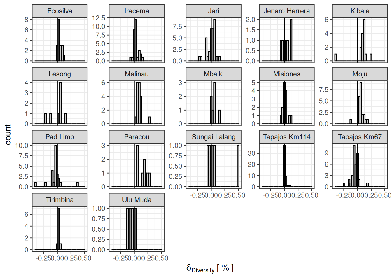
pars %>% 
  ggplot(aes(median.x)) +
  geom_histogram(fill = "lightgrey", col = "black") +
  geom_vline(xintercept = 0) +
  theme_bw() +
  facet_wrap(~ site, scales = "free_y") +
  xlab(expression(delta[Diversity] ~ "[ % ]"))

Code

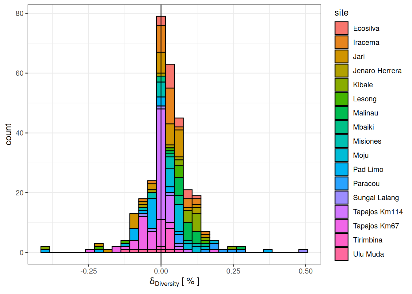
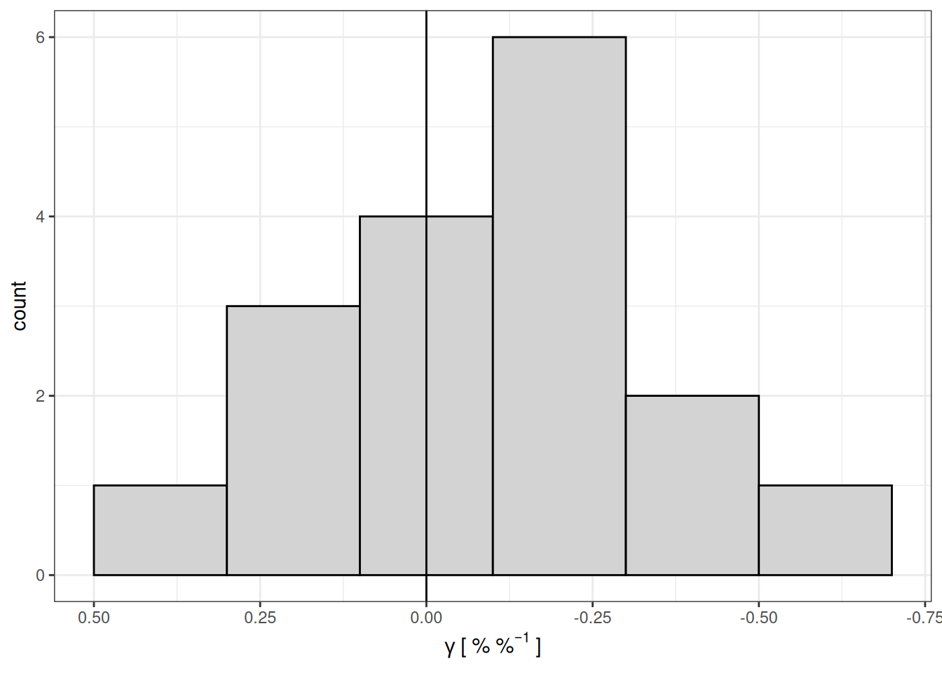
pars %>% 
  ggplot(aes(median.x)) +
  geom_histogram(aes(fill = site), col = "black") +
  geom_vline(xintercept = 0) +
  theme_bw() +
  xlab(expression(delta[Diversity] ~ "[ % ]"))

Code

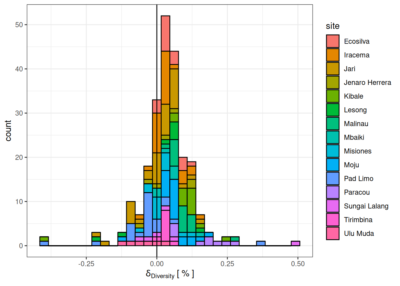
pars %>% 
  filter(!grepl("Tapajos", site)) %>% 
  ggplot(aes(median.x)) +
  geom_histogram(aes(fill = site), col = "black") +
  geom_vline(xintercept = 0) +
  theme_bw() +
  xlab(expression(delta[Diversity] ~ "[ % ]"))

IDH - H2

Code

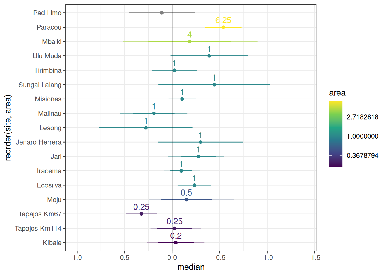
areas <- read_csv("data/raw_data/plot_area_v8.csv") %>% 
  rename(site_raw = Site) %>% 
  left_join(read_tsv("../modelling/data/raw_data/sites.tsv")) %>% 
  group_by(site) %>% 
  summarise(area = mean(PlotArea))

Rows: 625 Columns: 3
── Column specification ────────────────────────────────────────────────────────
Delimiter: ","
chr (2): Site, Plot
dbl (1): PlotArea

ℹ Use `spec()` to retrieve the full column specification for this data.
ℹ Specify the column types or set `show_col_types = FALSE` to quiet this message.
Rows: 144 Columns: 2
── Column specification ────────────────────────────────────────────────────────
Delimiter: "\t"
chr (2): site, site_raw

ℹ Use `spec()` to retrieve the full column specification for this data.
ℹ Specify the column types or set `show_col_types = FALSE` to quiet this message.
Joining with `by = join_by(site_raw)`

Code

read_tsv("outputs/gamma_gen_joint.tsv") %>% 
  left_join(areas) %>% 
  ggplot(aes(median, reorder(site, area), col = area)) +
  geom_point() +
  geom_text(aes(label = area), nudge_y = 0.5) +
  theme_bw() +
  scale_color_viridis_c(trans = "log") +
  geom_segment(aes(x = median - sd, xend = median + sd)) +
  geom_segment(aes(x = q5, xend = q95), size = .1) +
  geom_vline(xintercept = 0) +
  scale_x_reverse()

Rows: 17 Columns: 11
── Column specification ────────────────────────────────────────────────────────
Delimiter: "\t"
chr (2): variable, site
dbl (9): mean, median, sd, mad, q5, q95, rhat, ess_bulk, ess_tail

ℹ Use `spec()` to retrieve the full column specification for this data.
ℹ Specify the column types or set `show_col_types = FALSE` to quiet this message.
Joining with `by = join_by(site)`

Warning: Removed 1 row containing missing values or values outside the scale range
(`geom_text()`).

Code

fit$summary(c("gamma_s")) %>% 
  mutate(site = unique(ind$site)) %>% 
  write_tsv("outputs/gamma_gen_joint.tsv")
fit$draws(c("gamma_s")) %>% 
  mcmc_intervals() +
  scale_y_discrete(labels = unique(ind$site)) +
  scale_x_reverse(expression(gamma~"["~"%"~"%"^{-1}~"]"), lim = c(4,-4)) 

Posterior of the parameter gamma representing basal are disturbance intensity effect on genus diversity short term increase

Code

pars <- ind %>% 
  left_join(fit$summary(c("delta0_s"), "median") %>% 
              separate(variable, c("parameter", "s", "sitenum"), convert = TRUE) %>% 
              select(-s) %>% 
              pivot_wider(names_from = parameter, values_from = median)) %>% 
  left_join(fit$summary("gamma_s") %>% 
              separate(variable, c("parameter", "s", "sitenum"), convert = TRUE) %>% 
              select(-s) %>% 
              pivot_wider(names_from = parameter, values_from = median)) %>% 
  left_join(fit$summary(c("phi_ba_p", "delta_p"), "median") %>% 
              mutate(variable = gsub("phi_ba_p", "phiba_p", variable)) %>% 
              separate(variable, c("parameter", "p", "plotnum"), convert = TRUE) %>% 
              select(-p) %>% 
              pivot_wider(names_from = parameter, values_from = median))
pars %>% 
  ggplot(aes((1-phiba), delta)) +
  facet_wrap(~ site) +
  geom_abline(aes(slope = -mean, 
                  intercept = mean+delta0, group = site), 
              data = pars) +
    geom_abline(aes(slope = -mean-sd, 
                  intercept = mean-sd+delta0, group = site), 
              data = pars, linetype = "dashed") +
  geom_abline(aes(slope = -mean+sd, 
                  intercept = mean+sd+delta0, group = site), 
              data = pars, linetype = "dashed") +
  geom_point() +
  theme_bw() +
  xlab(expression(phi[BA] ~ "[ % lost ]")) +
  ylab(expression(delta[Diversity] ~ "[ % ]")) +
  theme(panel.spacing = unit(0, "lines")) +
  scale_x_continuous(labels = ~.*100) +
  scale_y_continuous(labels = ~.*100)

Inferred relationship between disturbance intensity and diversity short term increase.

Code

fit$summary(c("gamma_s")) %>% 
  ggplot(aes(median)) +
  geom_histogram(fill = "lightgrey", col = "black", binwidth = 0.2) +
  geom_vline(xintercept = 0) +
  theme_bw() +
  scale_x_reverse(expression(gamma~"["~"%"~"%"^{-1}~"]"))

Code

pars %>% 
  mutate(phi_ba = as.factor(round(phiba, 1))) %>% 
  ggplot(aes(phi_ba, abs(delta))) +
  geom_boxplot() +
  geom_violin() +
  geom_jitter() +
  theme_bw()

Code

pars %>% 
  ggplot(aes(phiba, delta, col = site)) +
  geom_point() +
  theme_bw()