Flux data

Code

library(tidyverse)
library(knitr)

Choice of variables

Below we show the productivity in four sites that have been remeasured for multiple decades.

Code

data <- read.csv("data/derived_data/aggregated_data_v9.csv") |>
  mutate(plot_new = Plot) |>
  separate(Plot, "Plot", "_")
plot_info <- read.csv("data/raw_data/bioforest-plot-information.csv")

Code

data |>
  left_join(plot_info, by = join_by(Site == site, Plot == plot)) |>
  subset(variable %in% c("agb_growth", "agb_recr")) |>
  subset(Site %in% c("Mbaiki", "Paracou", "Ulu Muda", "Lesong")) |>
  pivot_wider(names_from = "variable") |>
  ggplot(aes(Year, agb_recr + agb_growth, ,
    group = plot_new,
    col = Treatment
  )) +
  geom_point() +
  geom_line() +
  labs(y = "AGB productivity [Mg/ha/yr]", col = NULL) +
  facet_wrap(~Site, scales = "free") +
  theme_minimal()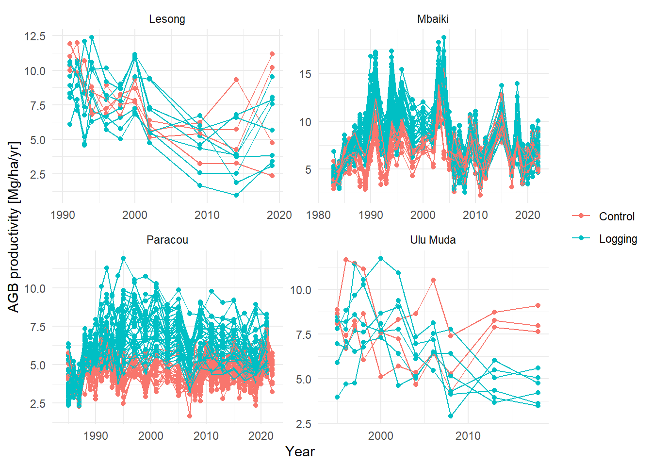

Code

data |>
  left_join(plot_info, by = join_by(Site == site, Plot == plot)) |>
  subset(variable == "nstem_recr") |>
  subset(Site %in% c("Mbaiki", "Paracou", "Ulu Muda", "Lesong")) |>
  ggplot(aes(Year, value, group = plot_new, col = Treatment)) +
  geom_point() +
  geom_line() +
  labs(y = "Stem recruitment [/ha/yr]", col = NULL) +
  facet_wrap(~Site, scales = "free") +
  theme_minimal()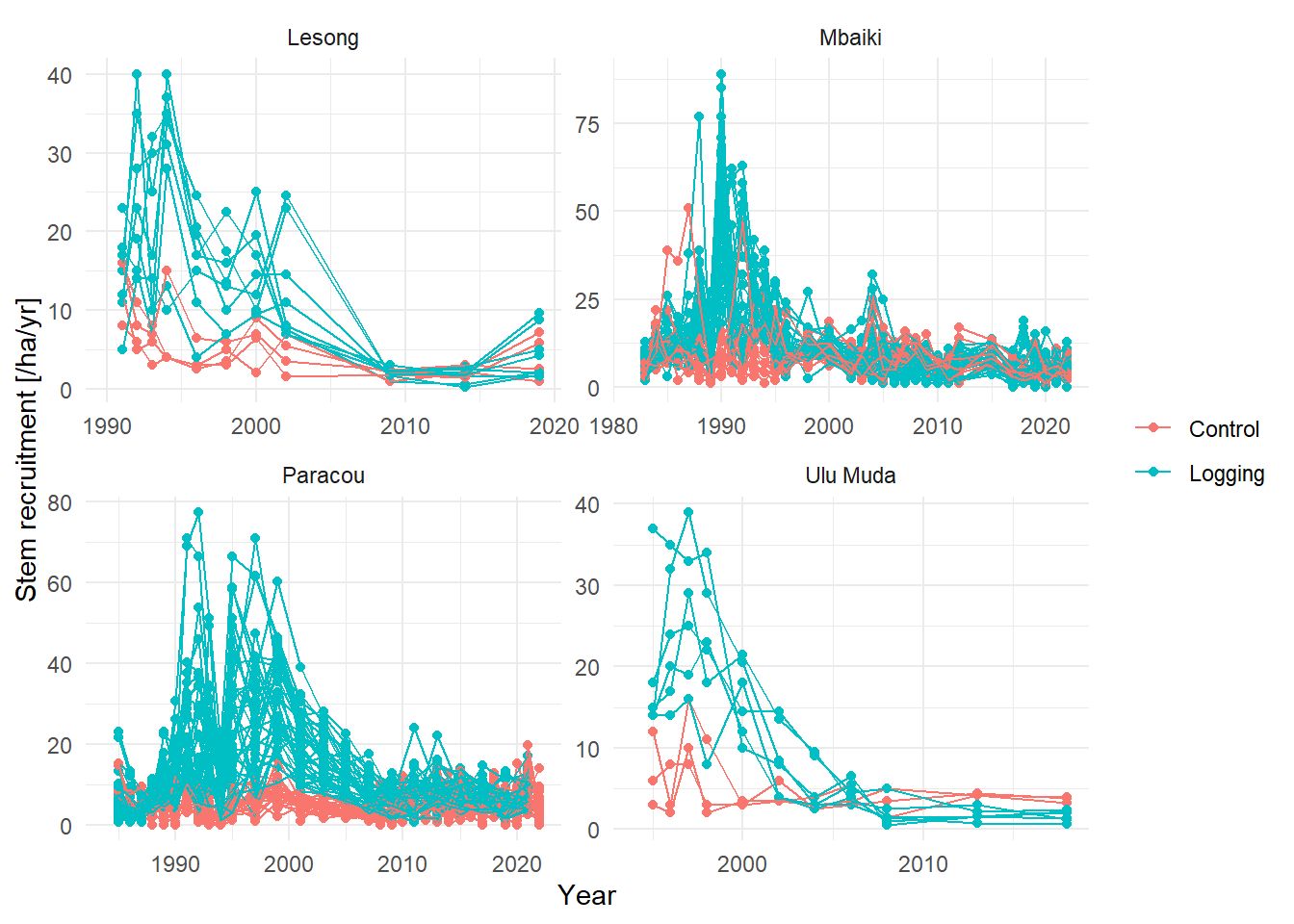

Code

data |>
  left_join(plot_info, by = join_by(Site == site, Plot == plot)) |>
  subset(variable == "agb_mort") |>
  filter(Treatment == "Control" | Year >= Year_of_harvest + 3) |>
  subset(Site %in% c("Mbaiki", "Paracou", "Ulu Muda", "Lesong")) |>
  ggplot(aes(Year, value, group = plot_new, col = Treatment)) +
  geom_point() +
  geom_line() +
  labs(y = "AGB mortality [Mg/ha/yr]", col = NULL) +
  facet_wrap(~Site, scales = "free") +
  theme_minimal()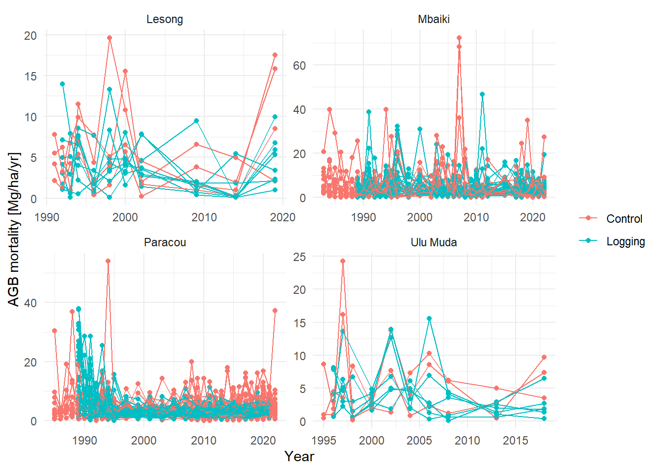

Code

data |>
  left_join(plot_info, by = join_by(Site == site, Plot == plot)) |>
  subset(variable == "nstem_mort") |>
  filter(Treatment == "Control" | Year >= Year_of_harvest + 3) |>
  subset(Site %in% c("Mbaiki", "Paracou", "Ulu Muda", "Lesong")) |>
  ggplot(aes(Year, value, group = plot_new, col = Treatment)) +
  geom_point() +
  geom_line() +
  labs(y = "Stem mortality [/ha/yr]", col = NULL) +
  facet_wrap(~Site, scales = "free") +
  theme_minimal()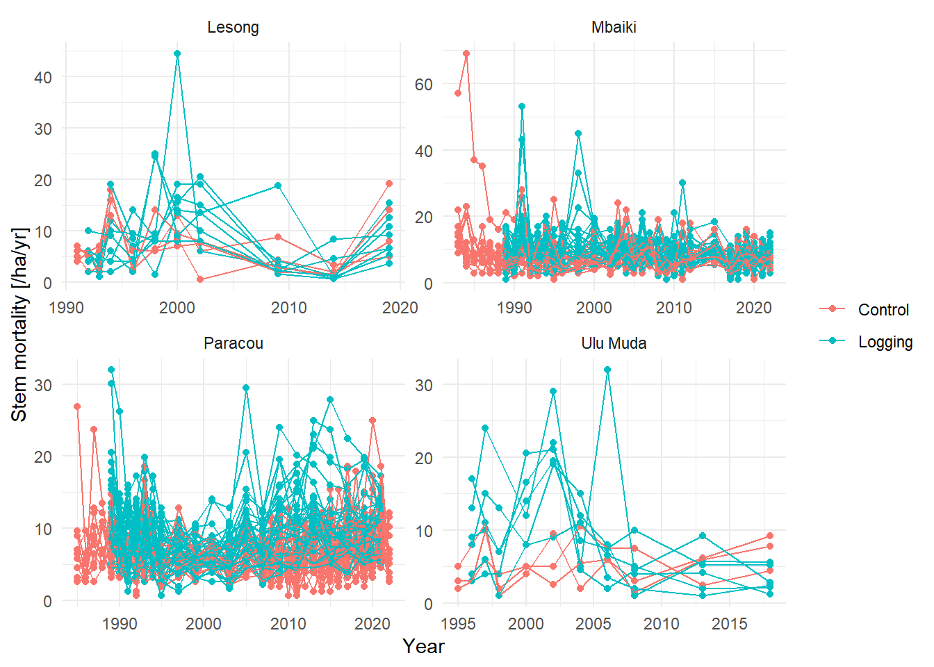

Site selection

In this analysis, we only kept sites that meet the following criteria:

at least 4 post-logging measurements
at least 10 years of post-logging measurements
presence of control plots
productivity values < 10% (too high)?

Code

criteria_site <- data |>
  inner_join(plot_info, by = join_by(Site == site, Plot == plot)) |>
  group_by(Site) |>
  summarise(
    controls = length(unique(plot_new[Treatment == "Control"])),
    logged = length(unique(plot_new[Treatment == "Logging"]))
  )
data |>
  inner_join(plot_info, by = join_by(Site == site, Plot == plot)) |>
  filter(Treatment == "Logging" & !is.na(Year)) |>
  group_by(Site, plot_new) |>
  summarise(
    ncensus = length(unique(Year[Year > Year_of_harvest])),
    tcensus = max(Year, na.rm = TRUE) - unique(Year_of_harvest)
  ) |>
  group_by(Site) |>
  summarise(ncensus = median(ncensus), tcensus = median(tcensus)) |>
  left_join(criteria_site) |>
  filter(ncensus > 3, tcensus > 9, controls > 0, logged > 0) |>
  write.csv("data/derived_data/sites_to_keep.csv", row.names = FALSE)

Code

read.csv("data/derived_data/sites_to_keep.csv") |>
  arrange(-ncensus) |>
  kable()

Site	ncensus	tcensus	controls	logged
Mbaiki	30	36.0	12	28
Paracou	22	35.0	24	36
Lesong	12	30.0	4	8
SUAS	12	24.0	4	16
Ulu Muda	12	25.0	3	6
Sungai Lalang	11	27.0	3	6
Tapajos Km67	11	36.0	18	48
Corinto	10	29.0	3	6
BAFOG	9	74.0	8	12
Jenaro Herrera	8	28.0	2	7
Jari	7	26.0	4	36
Misiones	7	19.5	4	14
Kibale	6	52.0	11	15
STREK	6	33.0	12	36
Kabo	4	33.0	3	9