Code
library(tidyverse)library(tidyverse)Here we define productivity and mortality as:
\[ flux(t) = \omega \cdot stocks(t) + \nu \cdot STP(t)\] where \(stocks(t)\) is the stocks value at time \(t\); \(\nu\) is either 0 (control plots) or 1 (logged plots).
The short term process (STP) is an intermediary process caused by logging operations, that disappears over time.
For productivity, we define it as: \(STP_P = \delta \cdot(\frac{t}{\tau}exp(1-\frac{t}{\tau}))^2\)
For mortality, we define it as \(STP_M = \alpha\cdot exp(-\lambda\cdot t)\)
Because we expect stocks to reach an equilibrium value at \(t \rightarrow +\infty\), we have:
\[lim_{+\infty}(prod) = lim_{+\infty}(mort)\] Therefore, \(\omega\) is the same for productivity and mortality.
We therefore have:
\[stocks(t) = stocks(0) + \int_0^t \left(\delta \cdot(\frac{x}{\tau}exp(1-\frac{x}{\tau}))^2 - \alpha\cdot exp(-\lambda\cdot x)\right)dx\]
The integral calculation is done in the Appendix.
The resulting stocks are:
\[ stocks(t) = stocks(0) + \frac{\delta \cdot e^{2} \cdot\tau}{4} - \delta \cdot e^{(1-\frac{t}{\tau})2} \left(\frac{t^2}{2\tau}+\frac{t}{2}+\frac{\tau}{4}\right) - \frac{\alpha}{\lambda}(1-exp(-\lambda\cdot t))\] The equilibrium value is
\[stocks(\infty) = stocks(0) + \frac{e^{2}}{4} (\delta \cdot \tau) - \frac{\alpha}{\lambda}\]
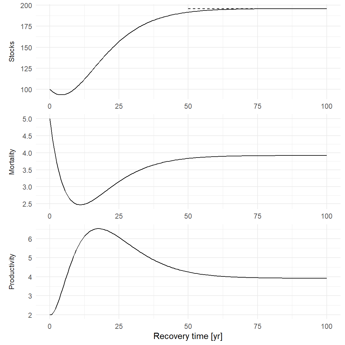
The figure below illustrates the resulting stocks and fluxes with parameters set to:
agb0 <- 100
tau <- 15
delta <- 4
alpha <- 3
lambda <- 0.2
omega <- 0.02

agbinf <- agb0 + exp(2) / 4 * delta * tau - alpha / lambda

stp <- function(time, delta, tau) {
  delta * (time / tau * exp(1 - time / tau))^2
}
stocks <- function(time, y0, delta, tau, lambda, alpha) {
  y0 + delta * tau * exp(2) / 4 -
    delta * exp((1 - time / tau) * 2) *
      (time^2 / (2 * tau) + time / 2 + tau / 4) -
    alpha / lambda * (1 - exp(-lambda * time))
}

facet_labs <- c(
  "agb" = "Stocks",
  "prod" = "Productivity",
  "mort" = "Mortality"
)
ann_segment <- data.frame(
  t = 50, tinf = 100, value = agbinf, name = "agb"
)

data.frame(t = seq(0, 100, length.out = 200)) |>
  mutate(
    prod = stp(t, delta, tau) +
      omega * stocks(t, agb0, delta, tau, lambda, alpha),
    mort = alpha * exp(-lambda * t) +
      omega * stocks(t, agb0, delta, tau, lambda, alpha),
    agb = stocks(t, agb0, delta, tau, lambda, alpha)
  ) |>
  pivot_longer(-t) |>
  ggplot(aes(t, value)) +
  geom_segment(data = ann_segment, aes(xend = tinf), lty = 2) +
  geom_line() +
  facet_wrap(~name,
    scales = "free", nrow = 3,
    labeller = labeller(name = facet_labs),
    strip.position = "left"
  ) +
  labs(x = "Recovery time [yr]", y = NULL) +
  theme_minimal() +
  theme(strip.placement = "outside")