Data
Code
<- read.csv ("data/raw_data/bioforest-plot-information.csv" ) |> select (site, plot, Year_of_harvest, Treatment)<- read.csv ("data/derived_data/aggregated_data_v9.csv" ) |> mutate (plot_new = Plot) |> separate (Plot, "Plot" , "_" ) |> left_join (plot_info, by = join_by (Site == site, Plot == plot)) |> filter (grepl ("^agb" , variable)) |> pivot_wider (names_from = "variable" , values_from = "value" ) |> mutate (prod = agb_growth + agb_recr, mort = agb_mort, stocks = agb) |> select (! contains ("agb" )) |> pivot_longer (cols = c ("stocks" , "prod" , "mort" ), names_to = "variable" ) |> mutate (Year_of_harvest = ifelse (Site == "Mbaiki" & Treatment == "Logging" ,1985 , Year_of_harvest|> mutate (trec = Year - Year_of_harvest)
For now, we only calibrate the model with sites that meet all the criteria listed here , and that have at least 10 censuses.
Code
<- read.csv ("data/derived_data/sites_to_keep.csv" ) |> filter (ncensus >= 10 )<- data |> filter (Site %in% sites$ Site)
Model
We used the following parameter bounds when calibrating the model.
Code
<- data.frame ("theta_min" = 50 ,"theta_max" = 1000 ,"lambda_min" = 1e-2 ,"lambda_max" = 5 ,"alpha_min" = 0 ,"alpha_max" = 200 ,"delta_min" = 0 ,"delta_max" = 20 ,"tau_min" = 2 ,"tau_max" = 30 ,"omega_min" = 1e-3 ,"omega_max" = 0.5 ,"y0_min" = 10 ,"y0_max" = 1000 |> pivot_longer (everything (), names_to = "parameter" ) |> separate (parameter, c ("parameter" , "bound" )) |> pivot_wider (names_from = bound) |> flextable ()
parameter
min
max
theta
50.000
1,000.0
lambda
0.010
5.0
alpha
0.000
200.0
delta
0.000
20.0
tau
2.000
30.0
omega
0.001
0.5
y0
10.000
1,000.0
Code
<- data |> mutate (sitenum = as.numeric (as.factor (Site))) |> subset (Treatment == "Logging" & trec > 3 ) |> pivot_wider (names_from = "variable" , values_from = "value" ) |> subset (! is.na (prod) & ! is.na (mort)) |> mutate (plotnum = as.numeric (as.factor (paste (Site, plot_new))))<- data |> mutate (sitenum = as.numeric (as.factor (Site))) |> subset (Treatment == "Control" | trec < 0 ) |> pivot_wider (names_from = "variable" , values_from = "value" ) |> subset (! is.na (prod) & ! is.na (mort))
Code
<- data_rec |> select (Site, Plot, sitenum, plotnum) |> unique () |> arrange (plotnum)<- list (n_equ = nrow (data_old),n_log = nrow (data_rec),s = max (data_old$ sitenum),p_log = max (data_rec$ plotnum),y_equ = data_old$ stocks,in_equ = data_old$ prod,out_equ = data_old$ mort,y_log = data_rec$ stocks,in_log = data_rec$ prod,out_log = data_rec$ mort,time = data_rec$ trec,site_equ = data_old$ sitenum,site_log = data_rec$ sitenum,plot_log = data_rec$ plotnum,site_plot = ind_rec$ sitenum,theta_bounds = c (bounds$ theta_min, bounds$ theta_max),lambda_bounds = c (bounds$ lambda_min, bounds$ lambda_max),alpha_bounds = c (bounds$ alpha_min, bounds$ alpha_max),delta_bounds = c (bounds$ delta_min, bounds$ delta_max),tau_bounds = c (bounds$ tau_min, bounds$ tau_max),omega_bounds = c (bounds$ omega_min, bounds$ omega_max),y0_bounds = c (bounds$ y0_min, bounds$ y0_max)sample_model ("flux_all" , mdata_all)
The resulting Stan fit summary is presented below.
Code
<- as_cmdstan_fit (list.files ("chains/flux_all/" , full.names = TRUE )
variable mean median sd mad q5 q95 rhat ess_bulk ess_tail
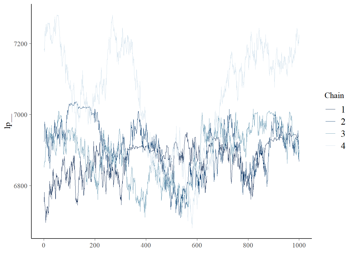
lp__ 7039.36 7031.27 78.60 82.12 6928.00 7181.21 1.35 9 26
mu_y0 355.39 354.87 6.18 6.66 346.58 366.01 1.07 44 441
sigma_y0 19.72 19.65 0.52 0.46 18.92 20.62 1.02 1149 1637
y0_p[1] 373.63 372.63 14.30 15.00 352.71 398.15 1.03 89 1564
y0_p[2] 349.68 348.19 13.89 12.35 326.38 373.04 1.02 218 367
y0_p[3] 338.83 339.91 13.63 13.03 314.71 360.31 1.02 214 621
y0_p[4] 358.32 356.63 13.36 12.34 336.40 381.53 1.03 650 1493
y0_p[5] 350.10 349.98 15.20 17.22 329.15 376.08 1.05 53 424
y0_p[6] 350.93 351.35 15.64 17.19 327.90 377.04 1.06 40 271
y0_p[7] 323.11 324.72 14.00 13.01 295.73 343.77 1.13 21 12
# showing 10 of 7128 rows (change via 'max_rows' argument or 'cmdstanr_max_rows' option)
Code
mcmc_trace (fit_flux_all$ draws (variables = c ("lp__" )))
The main parameter values are consistent with our expectations.
Code
c ("lambda_s" , "tau_s" , "theta_s" , "omega_s" ) |> $ summary () |> separate (variable, c ("variable" , NA , "sitenum" )) |> mutate (sitenum = as.numeric (sitenum)) |> left_join (unique (data_old[, c ("sitenum" , "Site" )])) |> select (variable, Site, mean, median, q5, q95, rhat)
# A tibble: 32 × 7
   variable Site           mean median    q5   q95  rhat
   <chr>    <chr>         <dbl>  <dbl> <dbl> <dbl> <dbl>
 1 lambda   Corinto       1.82   1.81  1.53  2.16   1.04
 2 lambda   Lesong        0.868  0.862 0.797 0.950  1.13
 3 lambda   Mbaiki        1.70   1.70  1.53  1.86   1.04
 4 lambda   Paracou       1.59   1.58  1.42  1.72   1.09
 5 lambda   SUAS          4.72   4.79  4.15  4.99   1.09
 6 lambda   Sungai Lalang 0.788  0.786 0.734 0.846  1.09
 7 lambda   Tapajos Km67  1.30   1.30  1.19  1.39   1.06
 8 lambda   Ulu Muda      0.835  0.829 0.776 0.900  1.03
 9 tau      Corinto       4.82   4.85  3.74  5.90   1.04
10 tau      Lesong        7.62   7.61  6.95  8.20   1.04
# ℹ 22 more rows
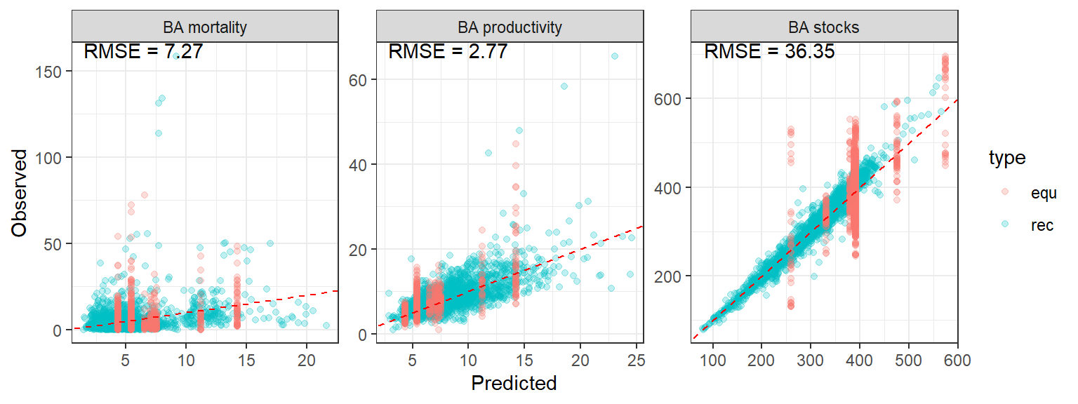
The goodness of fit is satisfactory.
Code
<- data_rec |> select (- plotnum) |> mutate (stocks = fit_flux_all$ summary (c ("mu_y_log" ), median)$ median,prod = fit_flux_all$ summary (c ("mu_in_log" ), median)$ median,mort = fit_flux_all$ summary (c ("mu_out_log" ), median)$ median,val = "pred" ,type = "rec" |> rbind (mutate (stocks = $ summary (c ("theta_s" ), median)$ median[data_old$ sitenum],prod = fit_flux_all$ summary (c ("theta_s" ), median)$ median[data_old$ sitenum] * $ summary (c ("omega_s" ), median)$ median[data_old$ sitenum], # nolint mort = fit_flux_all$ summary (c ("theta_s" ), median)$ median[data_old$ sitenum] * $ summary (c ("omega_s" ), median)$ median[data_old$ sitenum], # nolint val = "pred" ,type = "equ" <- data_rec |> mutate (val = "obs" ,type = "rec" |> select (- plotnum) |> rbind (mutate (val = "obs" ,type = "equ" <- rbind (pred_data, obs_data) |> pivot_longer (cols = c (stocks, prod, mort), names_to = "variable" ) |> pivot_wider (names_from = val, values_from = value)<- pov_data |> group_by (variable) |> summarise (rmse = sqrt (mean ((pred - obs)^ 2 )))<- c (stocks = "BA stocks" , prod = "BA productivity" , mort = "BA mortality" )|> ggplot (aes (pred, obs)) + geom_point (alpha = 0.25 , aes (col = type)) + geom_abline (col = "red" , linetype = "dashed" ) + geom_text (data = df_rmse,aes (x = - Inf , y = Inf , hjust = - 0.1 , vjust = 1 ,label = paste ("RMSE =" , round (rmse, 2 ))+ theme_bw () + xlab ("Predicted" ) + ylab ("Observed" ) + facet_wrap (~ variable, scales = "free" , labeller = labeller (variable = labs))
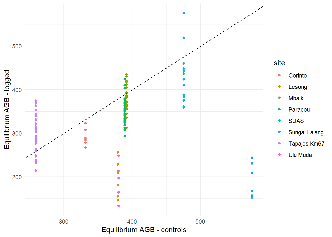
The equilibrium AGB estimated in the logged plots is consistent overall with the control plots, except in the Malaysian sites (Lesong, Sungai Lalang and Ulu Muda), where it is significantly lower.
Code
<- data_rec |> select (Site, Plot, sitenum, plotnum) |> unique () |> arrange (plotnum)data.frame (site = levels (as.factor (data_old$ Site))[ind_rec$ sitenum],theta_rec = fit_flux_all$ summary (c ("theta_log" ), median)$ median,theta_equ = $ summary (c ("theta_s" ), median)$ median[ind_rec$ sitenum]|> ggplot (aes (theta_equ, theta_rec, col = site)) + geom_point () + geom_abline (intercept = 0 , slope = 1 , lty = 2 ) + labs (x = "Equilibrium AGB - controls" , y = "Equilibrium AGB - logged" ) + theme_minimal ()
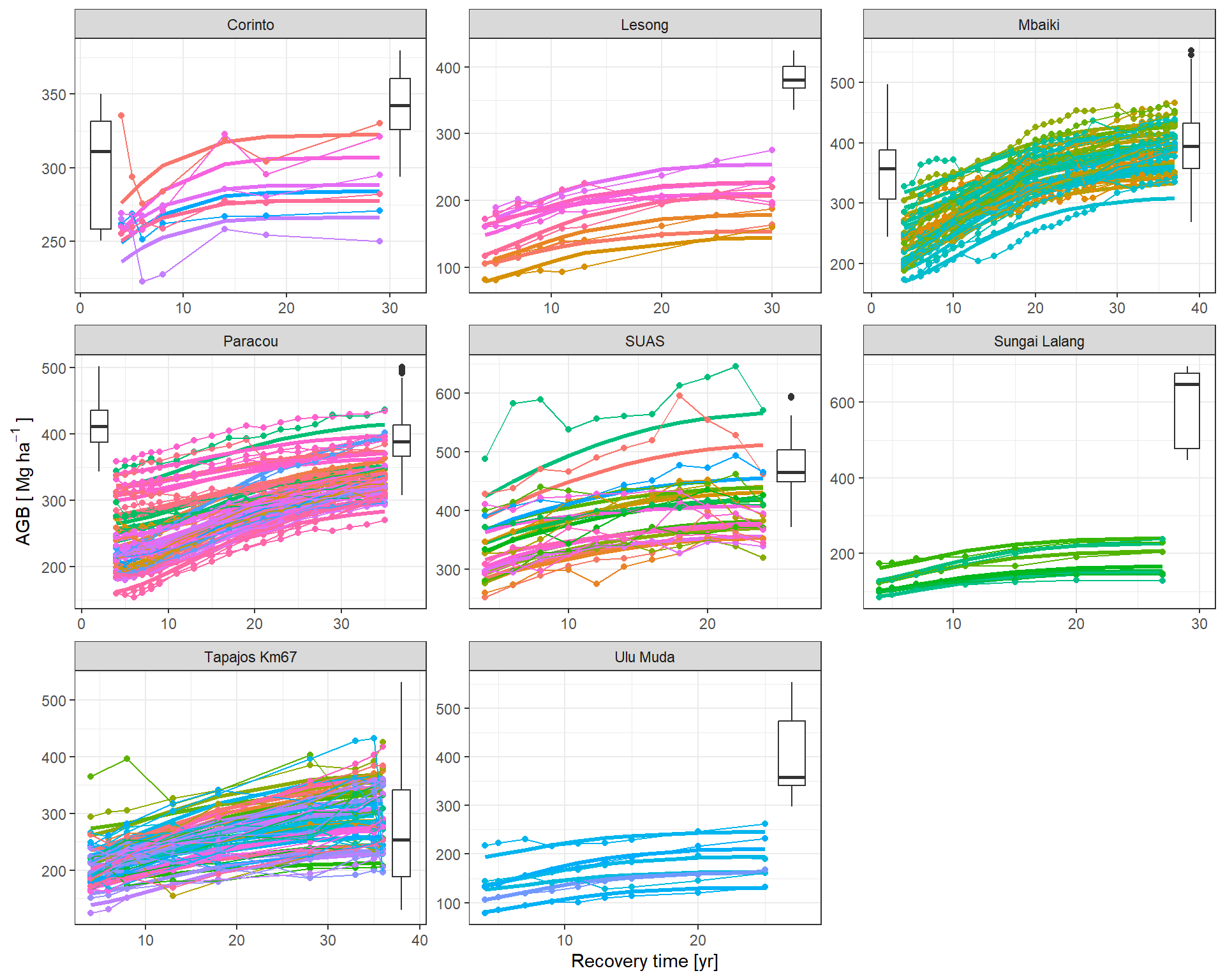
Visualising the trajectories
The predicted flux and stocks trajectories look consistent with the data.
Code
|> subset (variable == "stocks" ) |> mutate (Plot = plot_new) |> graph_traj (expression ("AGB [" ~ Mg ~ ha^- 1 ~ "]" ))
Code
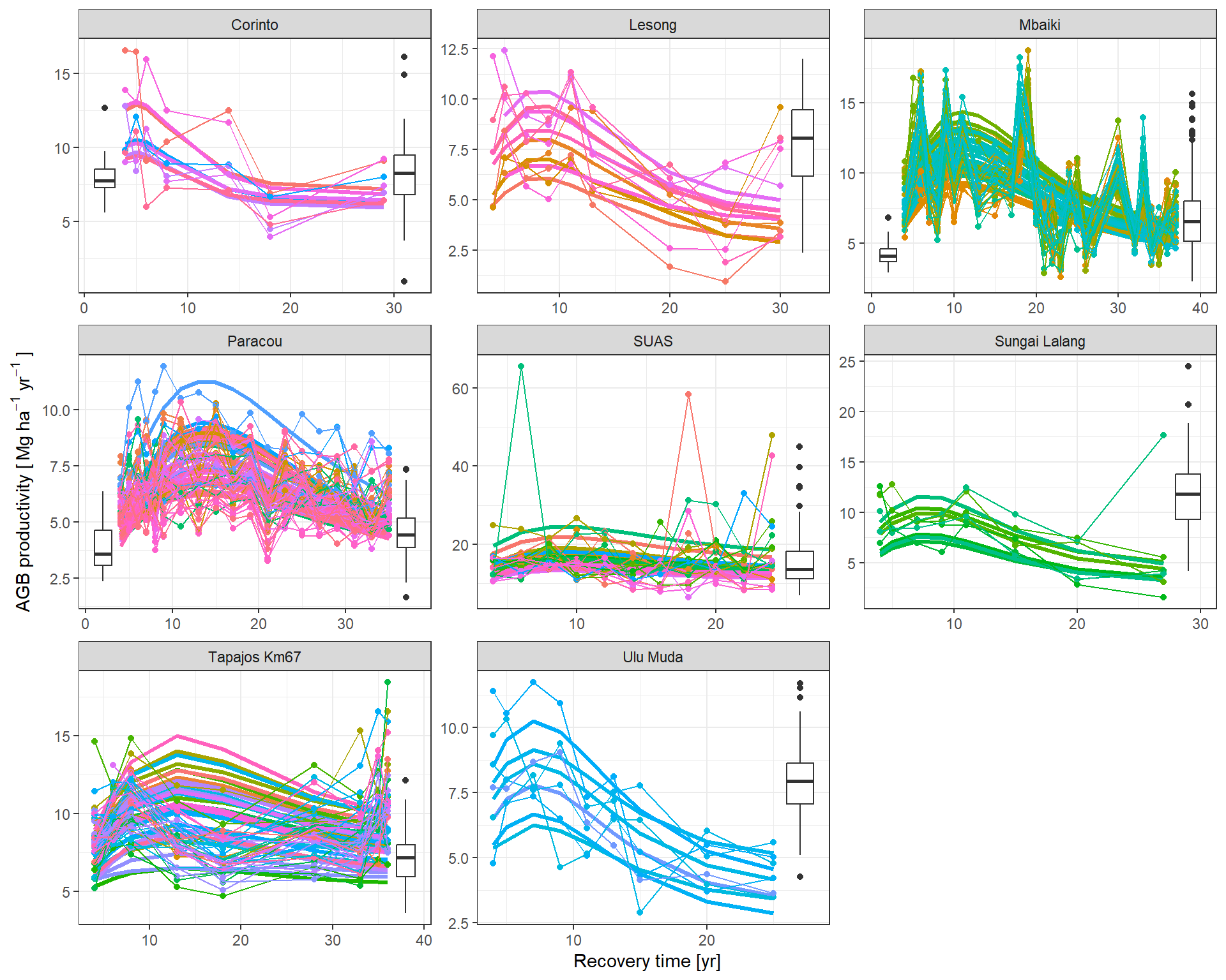
|> subset (variable == "prod" ) |> mutate (Plot = plot_new) |> graph_traj (expression ("AGB productivity [" ~ Mg ~ ha^- 1 ~ yr^- 1 ~ "]" ))
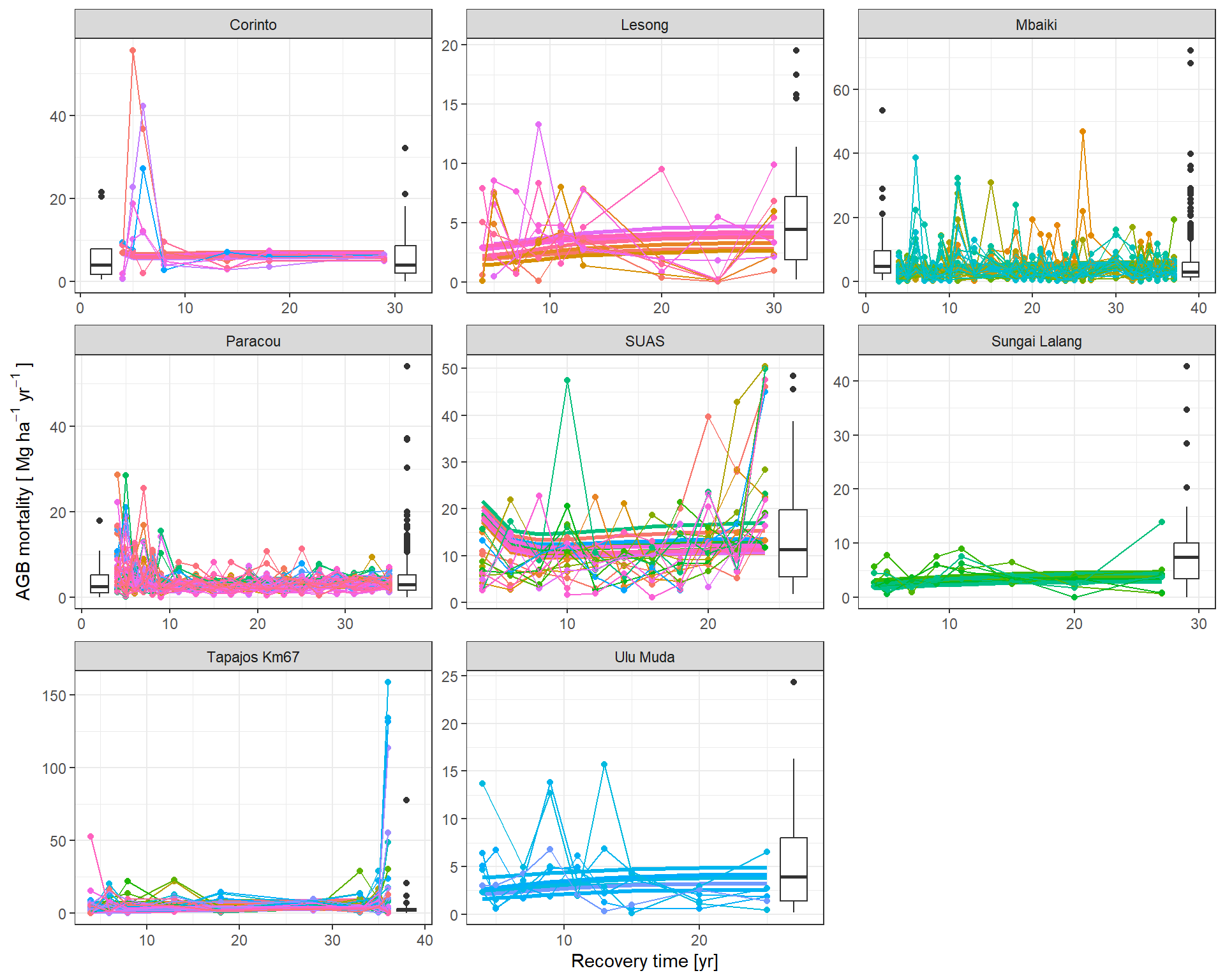
Code
|> subset (variable == "mort" ) |> mutate (Plot = plot_new) |> graph_traj (expression ("AGB mortality [" ~ Mg ~ ha^- 1 ~ yr^- 1 ~ "]" ))