Sites

This page describes all sites and plots coordinates preparation and visualization.

First we had to prepare WGS84 - World Geodetic System 1984 coordinates from WGS 84 UTM zone 21N for Iwokrama.

Code

sites %>%
  mutate(plot = as.character(plot)) %>%
  unnest(plot) %>%
  filter(site == "Iwokrama") %>%
  select(
    plot,
    `Location (WGS UTM 21N) SW corners...5`,
    `Location (WGS UTM 21N) SW corners...6`
  ) %>%
  rename(
    lat = `Location (WGS UTM 21N) SW corners...5`,
    lon = `Location (WGS UTM 21N) SW corners...6`
  ) %>%
  sf::st_as_sf(coords = c("lat", "lon"), crs = "EPSG:32621") %>%
  sf::st_transform(4326) %>%
  sf::st_coordinates() %>%
  as_data_frame() %>%
  write_tsv("test.tsv")

Code

sites <- googlesheets4::read_sheet("https://docs.google.com/spreadsheets/d/1fq2owxMBLBwwibcdw2uQQFxnIhsMbaH4Qcj_xUwVvSQ/edit?gid=0#gid=0") %>% #nolint
  mutate(plot = as.character(plot)) %>%
  unnest(plot) %>%
  select(site, plot, latitude, longitude) %>%
  na.omit() %>%
  write_tsv("outputs/sites.tsv")

We obtained the following sites and plots distribution globally.

Other sites location might unprecised and should be checked against forest landscape data.

Code

read_tsv("outputs/sites.tsv") %>%
  st_as_sf(coords = c("longitude", "latitude"), crs = 4326) %>%
  leaflet() %>%
  addTiles() %>%
  addMarkers(label = ~ paste(site, plot),
             labelOptions = labelOptions(noHide = FALSE))

Sites and plots locations.

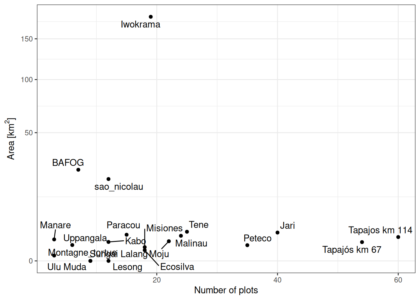
Most sites showed a small dispersion of plots covering up 10 km² at the exception of BAFOG & Sao Nicolau covering tenth of km² and Iwokrama covering more than 150 km² .

Code

read_tsv("outputs/sites.tsv") %>%
  st_as_sf(coords = c("longitude", "latitude"), crs = 4326) %>%
  group_by(site) %>%
  summarise(n = n()) %>%
  st_convex_hull() %>%
  mutate(area = as.numeric(set_units(st_area(.), "km^2"))) %>%
  st_drop_geometry() %>%
  ggplot(aes(n, area)) +
  geom_point() +
  theme_bw() +
  xlab("Number of plots") +
  ylab(expression(paste("Area [", km^2, "]"))) +
  ggrepel::geom_text_repel(aes(label = site)) +
  scale_y_sqrt()

Number of sites and total plots surface.