Climate

We retrieved all data from TerraClimate (Abatzoglou et al. 2018). The variables are extracted for each plot of each site and every month from 1958 to 2023. The raw variables are:

ET: Actual evapotranspiration, mm
CWD: Climate water deficit, mm
Tmax: Maximum temperature, °C
Tmin: Minimum temperature, °C
PDSI: Palmer Drought Severity Index
PET: Potential evapotranpiration, mm
Pr: precipitation, mm
Soil: Soil humidity, mm
VPD: Vapour Pressure Deficit, kPa

Code

all_dat <- list.files("data/derived_data/climate/", full.names = TRUE) %>%
  read_tsv() %>%
  group_by(site) %>%
  mutate(
    aet = aet * .1, def = def * .1, pdsi = pdsi * .01, pet = pet * .1,
    tmmn = tmmn * .1, tmmx = tmmx * .1, vpd = vpd * .01, soil = soil * .1
  ) %>%
  mutate(month = month(time)) %>%
  mutate(year = year(time))
monthly <- all_dat %>%
  select(site, month, pr, tmmn, tmmx, soil) %>%
  group_by(site, month) %>%
  summarise_all(mean)
write_tsv(monthly, "data/derived_data/climate_month.tsv")
ds <- all_dat %>%
  filter(aet > pr) %>%
  group_by(site, year) %>%
  summarise(dsl = n() * 30, dsi = sum(aet - pr)) %>%
  select(-year) %>%
  group_by(site) %>%
  summarise_all(mean)
yearly <- all_dat %>%
  group_by(site, year) %>%
  summarise(
    et = sum(aet),
    cwd = sum(def),
    pr = sum(pr),
    tmax = max(tmmx),
    vpd = max(vpd),
    soil = min(soil)
  ) %>%
  select(-year) %>%
  group_by(site) %>%
  summarise_all(mean) %>%
  left_join(ds)
write_tsv(yearly, "data/derived_data/climate_year.tsv")

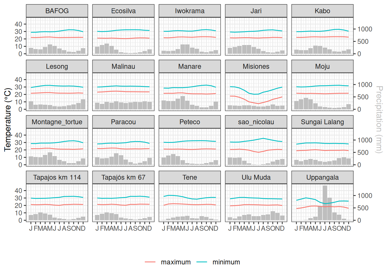
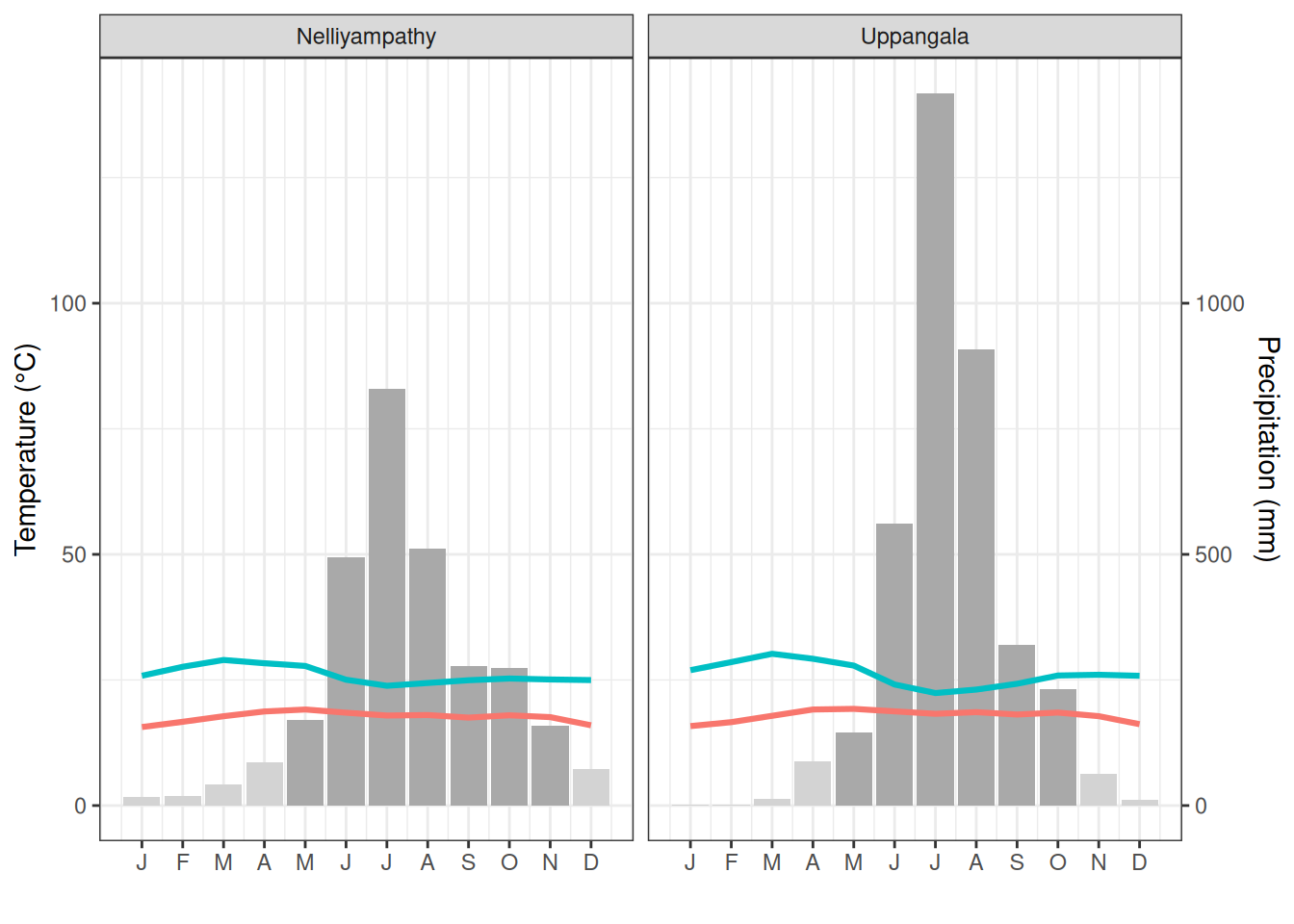
For a quick exploration of each site climatology we first had a look to umbrothermal diagrams for the mean climate of each site, opposing for instance highly seasonal monsoon regimes from India un Uppangala to less seasonal regimes from Misiones in Argentina.

Code

read_tsv("data/derived_data/climate_month.tsv") %>%
  filter(!(site %in% c("Uppangala", "Nelliyampathy"))) %>%
  group_by(site, month) %>%
  summarise_all(mean) %>%
  ggplot(aes(x = month)) +
  geom_col(aes(y = pr / 10, fill = pr < 100), col = NA) +
  geom_line(aes(y = tmmn, col = "maximum"), linewidth = 1.1) +
  geom_line(aes(y = tmmx, col = "minimum"), linewidth = 1.1) +
  theme_bw() +
  xlab("") +
  scale_x_continuous(
    breaks = 1:12,
    labels = c("J", "F", "M", "A", "M", "J", "J", "A", "S", "O", "N", "D")
  ) +
  scale_y_continuous(
    name = "Temperature (°C)",
    sec.axis = sec_axis(trans = ~ . * 10, name = "Precipitation (mm)")
  ) +
  scale_color_discrete(guide = "none") +
  facet_wrap(~site) +
  scale_fill_manual(guide = "none", values = c("darkgrey", "lightgrey"))

Umbrothermal diagrams for the mean climate of each site.

Code

read_tsv("data/derived_data/climate_month.tsv") %>%
  filter(site %in% c("Uppangala", "Nelliyampathy")) %>%
  group_by(site, month) %>%
  summarise_all(mean) %>%
  ggplot(aes(x = month)) +
  geom_col(aes(y = pr / 10, fill = pr < 100), col = NA) +
  geom_line(aes(y = tmmn, col = "maximum"), linewidth = 1.1) +
  geom_line(aes(y = tmmx, col = "minimum"), linewidth = 1.1) +
  theme_bw() +
  xlab("") +
  scale_x_continuous(
    breaks = 1:12,
    labels = c("J", "F", "M", "A", "M", "J", "J", "A", "S", "O", "N", "D")
  ) +
  scale_y_continuous(
    name = "Temperature (°C)",
    sec.axis = sec_axis(trans = ~ . * 10, name = "Precipitation (mm)")
  ) +
  scale_color_discrete(guide = "none") +
  facet_wrap(~site) +
  scale_fill_manual(guide = "none", values = c("darkgrey", "lightgrey"))

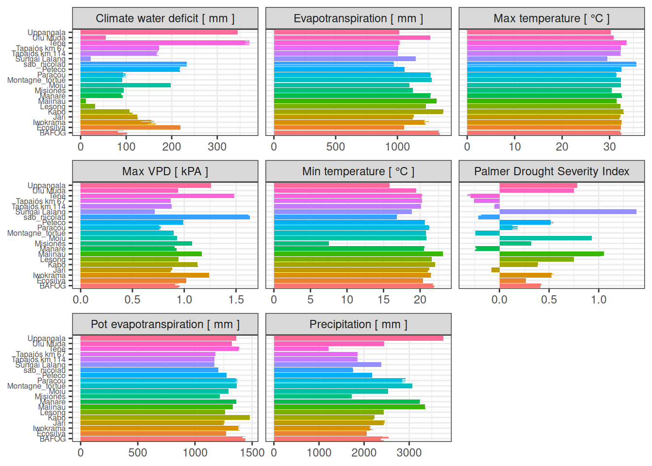
To ease plot and sites comparisons, we derived yearly metrics:

CWD: Climate water deficit, mm, mean across years of the sum of monthly CWD
ET: Evapotranspiration, mm, mean across years of the sum of monthly ET
Pr: Precipitation, mm, mean across years of the sum of monthly Pr
Soil: Soil humidity, mm, mean across years of the minimum of monthly soil humidity
VPD: Vapour Pressure Deficit, kPa, mean across years of the maximum of monthly VPD
Tmax: Maximum temperature, °C, mean across years of the maximum of monthly Tmax
DSL: Dry season length, days, mean across years of the number of month with ET>Pr multiplied by 30
DSI: Dry season intensity, mm, mean across years of the sum of ET-Pr for month with ET>Pr

This better revealed among sites differences with for instance highest dry season intensity and length at Uppangala despite highest total precipitation.

Code

read_tsv("data/derived_data/climate_year.tsv") %>%
  gather(variable, value, -site) %>%
  mutate(var_long = recode(variable,
    "et" = "Evapotranspiration [ mm ]",
    "cwd" = "Climate water deficit [ mm ]",
    "pr" = "Precipitation [ mm ]",
    "tmax" = "Max temperature [ °C ]",
    "vpd" = "Max VPD [ kPA ]",
    "soil" = "Min soil humidity [ mm ]",
    "dsi" = "Dry season intensity [ mm ]",
    "dsl" = "Dry season length [ day ]"
  )) %>%
  ggplot(aes(site, value, fill = site, group = site)) +
  geom_col(position = "dodge") +
  facet_wrap(~var_long, scales = "free_y") +
  theme_bw() +
  theme(
    legend.position = "bottom", axis.title = element_blank(),
    axis.text.x = element_blank(),
    legend.key.size = unit(0.5, "line")
  ) +
  scale_fill_discrete("")

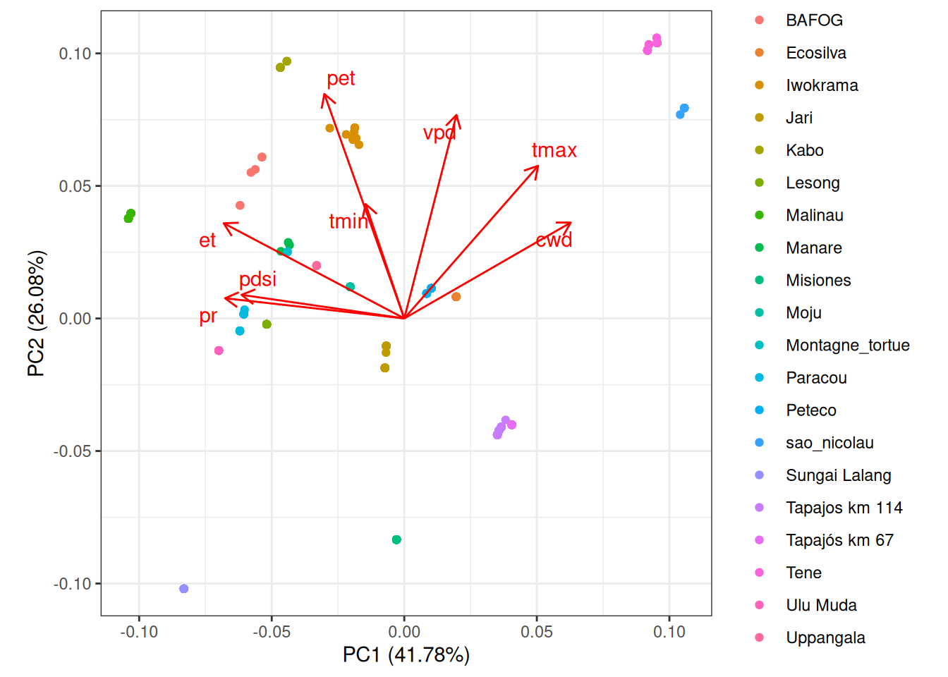
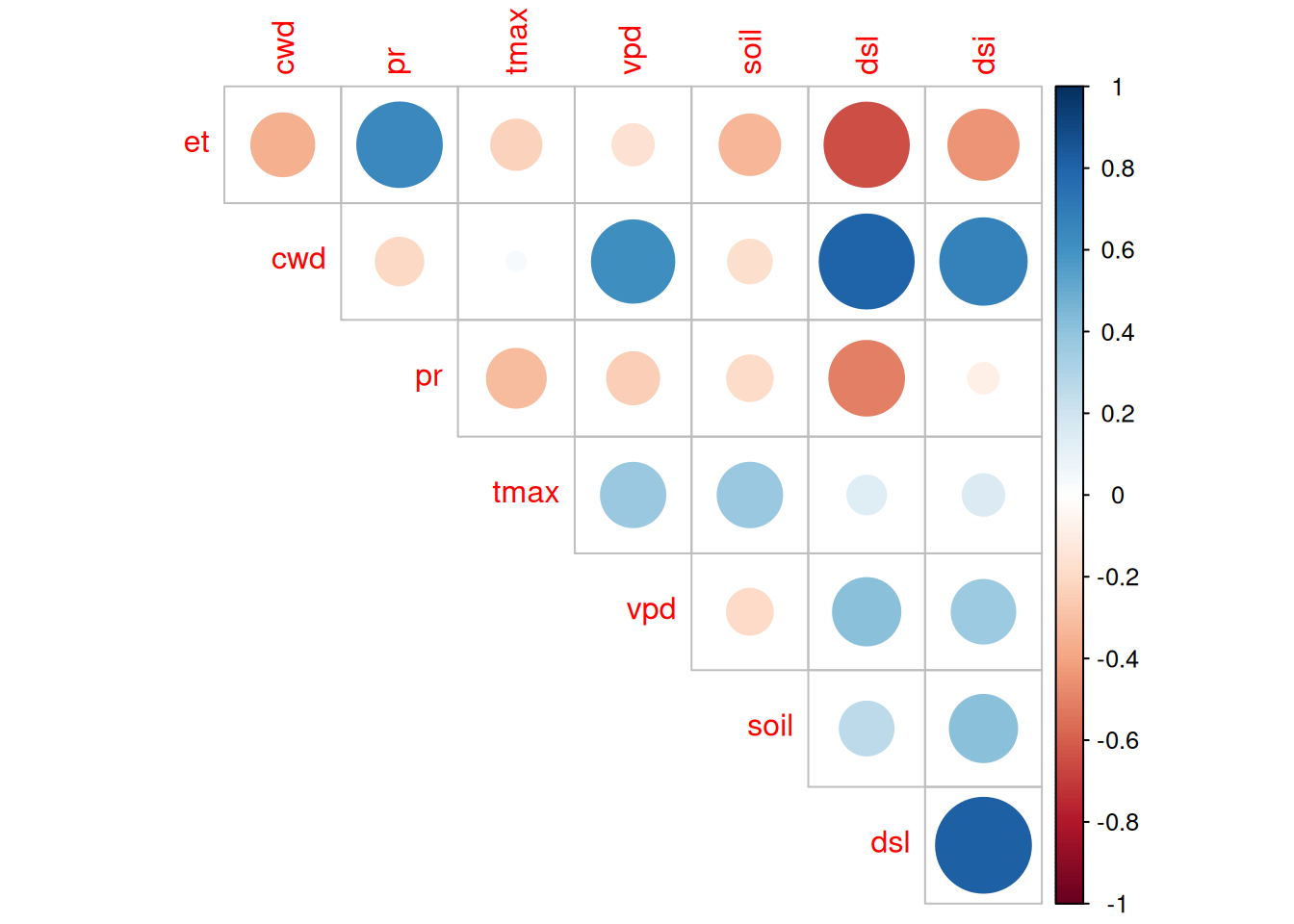
The first ordination axis retained almost half of the variations.

Code

data <- read_tsv("data/derived_data/climate_year.tsv")
pca <- prcomp(data %>% select(-site), scale. = TRUE)
autoplot(pca,
  loadings = TRUE, loadings.label = TRUE,
  loadings.label.repel = TRUE,
  data = data, colour = "site"
) +
  theme_bw() +
  coord_equal() +
  scale_color_discrete("") +
  theme(legend.key.size = unit(0.5, "line"))

Yearly mean climate variables PCA per site and plot.

Code

read_tsv("data/derived_data/climate_year.tsv") %>%
  select(-site) %>%
  cor(use = "pairwise.complete.obs") %>%
  corrplot::corrplot(type = "upper", diag = FALSE)

Climate variables pairwise correlations.

We will extract all for modelling but group 2 is focusing on climate stress which I think could be well represented by DSL, DSI, Soil and/or Tmax.