Metrics

Metrics gathering for modelling steps of the project:

• CWD: Climate water deficit, mm
• ET: Evapotranspiration, mm
• Pr: Precipitation, mm
• Soil: Soil humidity, mm
• VPD: Vapour Pressure Deficit, kPa
• Tmax: Maximum temperature, °C
• DSL: Dry season length, daysmultiplied by 30
• DSI: Dry season intensity, mm
• Clay: Proportion of clay, %
• Sand: Proportion of sand, %
• Silt: Proportion of silt, %
• BDOD: Bulk density, kg dm³
• CEC: Cation Exchange Capacity, cmolC kg^-1
• CF: Coarse Fragments , cm³ 100cm^-3
• N: Soil nitrogen, g kg^-1
• pH: Soil pH
• SOC: Soil organic carbon content, g kg^-1
• OCD: Organic carbon density, kg dm³

Code

sites <- read_tsv("data/derived_data/sites.tsv") %>% 
  select(-plot)
climate <- read_tsv("data/derived_data/climate_year.tsv")
soil <- read_tsv("data/derived_data/soil.tsv") %>%
  group_by(site) %>%
  filter(depth <= 15) %>%
  summarise_all(mean, na.omit = TRUE) %>%
  select(-X, -Y, -depth, -ocs)
sites %>%
  left_join(climate) %>%
  left_join(soil) %>%
  write_tsv("outputs/environment.tsv")

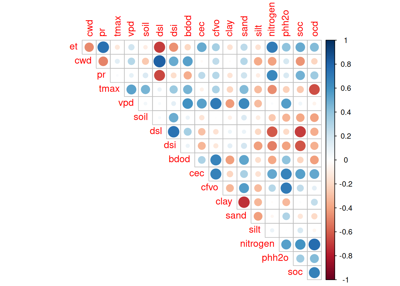
We have correlation among group of variables, notably among climate and soil, which is logical but should be taken into account. For instance SOC is highly anti-correlated to DSL and DSI.

Code

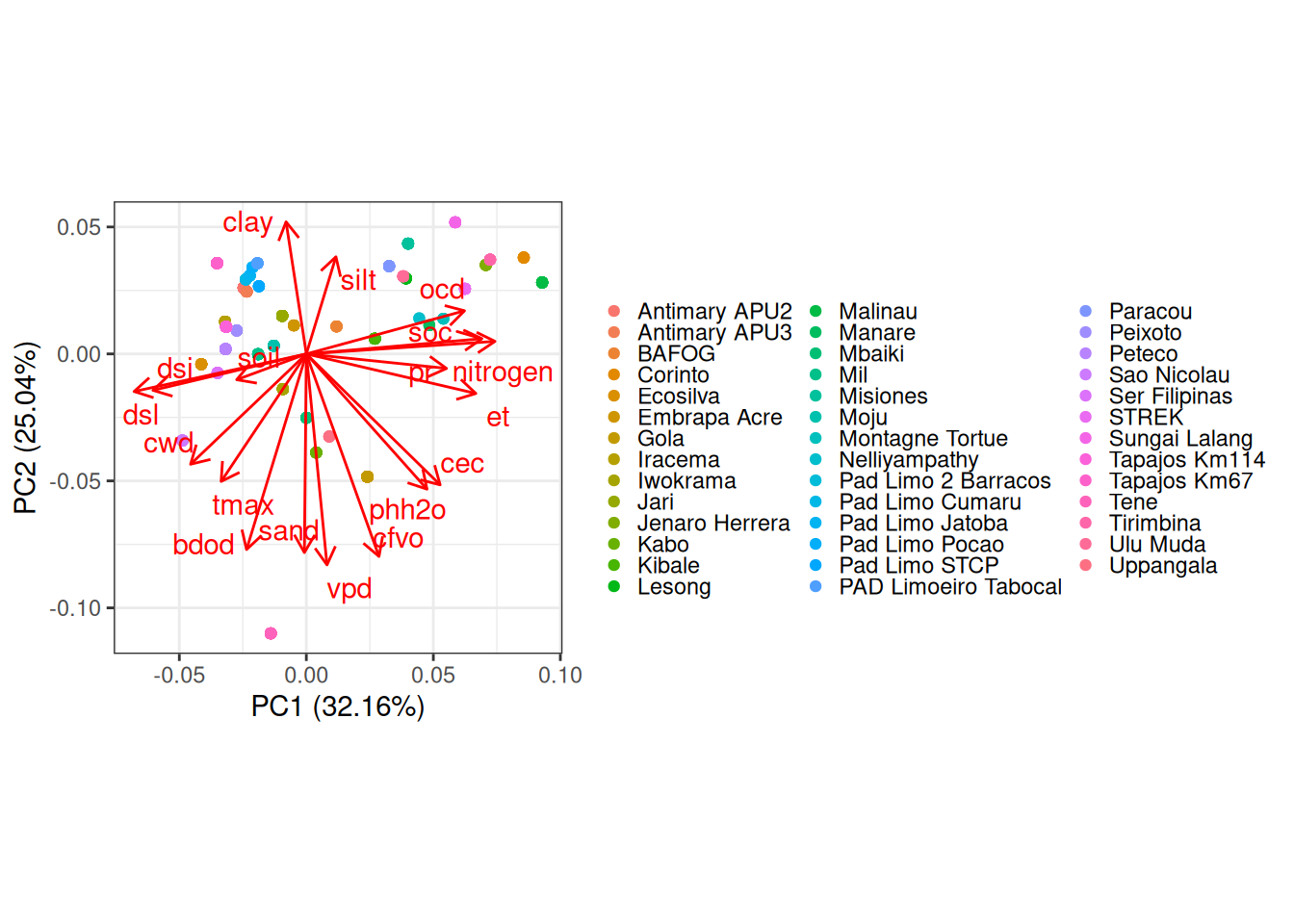
data <- read_tsv("outputs/environment.tsv") %>%
  na.omit()
pca <- prcomp(data %>% select(-site, -longitude, -latitude),
              scale. = TRUE)
autoplot(pca,
  loadings = TRUE, loadings.label = TRUE,
  loadings.label.repel = TRUE,
  data = data, colour = "site"
) +
  theme_bw() +
  coord_equal() +
  scale_color_discrete("") +
  theme(legend.key.size = unit(0.5, "line"))

All variables PCA per site and plot.

Code

read_tsv("outputs/environment.tsv") %>%
  select(-site, -longitude, -latitude) %>%
  cor(use = "pairwise.complete.obs") %>%
  corrplot::corrplot(type = "upper", diag = FALSE)

All variables pairwise correlations.