Soil

We retrieved all data from SoilGrids detailed below (Poggio et al. 2021):

Clay: Proportion of clay particles (< 0.002 mm) in the fine earth fraction, %
Sand: Proportion of sand particles (> 0.05 mm) in the fine earth fraction, %
Silt: Proportion of silt particles (≥ 0.002 mm and ≤ 0.05 mm) in the fine earth fraction, %
BD: Bulk density of the fine earth fraction, kg dm³
CEC: Cation Exchange Capacity of the soil, cmolC kg^-1
CF: Volumetric fraction of coarse fragments (> 2 mm), cm³ 100cm^-3
N: Total nitrogen, g kg^-1
pH: Soil pH
SOC: Soil organic carbon content in the fine earth fraction, g kg^-1
OCD: Organic carbon density, kg dm³
OCS: Organic carbon stocks, kg m²

Code

list.files("data/derived_data/soil/", full.names = TRUE) %>%
  read_tsv() %>%
  select(-time) %>%
  gather(variable, value, -site, -X, -Y) %>%
  separate(variable, c("variable", "depth"), "_") %>%
  separate(depth, c("mindepth", "depth"), "-") %>%
  mutate(depth = as.numeric(gsub("cm", "", depth))) %>%
  select(-mindepth) %>%
  pivot_wider(names_from = variable, values_from = value) %>%
  mutate(
    bdod = bdod / 100,
    cec = cec / 10,
    cfvo = cfvo / 10,
    clay = clay / 10,
    sand = sand / 10,
    silt = silt / 10,
    nitrogen = nitrogen / 100,
    phh2o = phh2o / 10,
    soc = soc / 10,
    ocd = ocd / 10,
    ocs = ocs / 10
  ) %>%
  write_tsv("data/derived_data/soil.tsv")

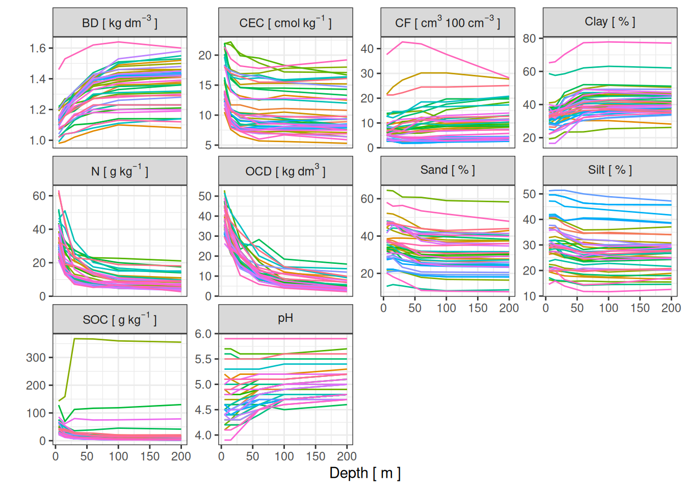
We have information per depth in each plot as shown below, I focused on the two top horizons (0-15cm) revealing most inter-site variations (V. Freycon pers. com.).

Code

read_tsv("data/derived_data/soil.tsv") %>%
  select(-X, -Y, -ocs) %>%
  gather(variable, value, -depth, -site) %>%
  mutate(var_long = recode(variable,
    "bdod" = '"BD ["~kg~dm^{-3}~"]"',
    "cec" = '"CEC ["~cmol~kg^{-1}~"]"',
    "cfvo" = '"CF ["~cm^3~"100"~cm^{-3}~"]"',
    "clay" = '"Clay ["~"%"~"]"',
    "nitrogen" = '"N ["~g~kg^{-1}~"]"',
    "ocd" = '"OCD ["~kg~dm^{3}~"]"',
    "phh2o" = "pH",
    "sand" = '"Sand ["~"%"~"]"',
    "silt" = '"Silt ["~"%"~"]"',
    "soc" = '"SOC ["~g~kg^{-1}~"]"'
  )) %>%
  ggplot(aes(depth, value, colour = site)) +
  geom_line() +
  facet_wrap(~var_long, scales = "free_y", labeller = label_parsed) +
  theme_bw() +
  ylab("") +
  xlab("Depth [ m ]") +
  scale_color_discrete(guide = "none")

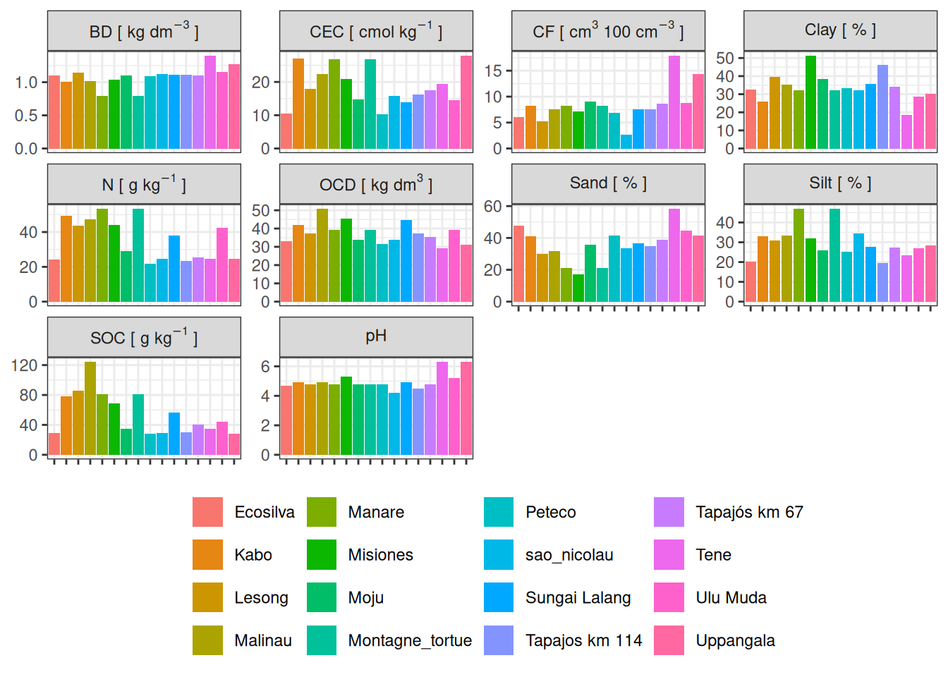
Soil data variation with depth at Paracou across plots.

The plots showed low variation within site but wider variation among sites.

Code

read_tsv("data/derived_data/soil.tsv") %>%
  select(-X, -Y) %>%
  group_by(site) %>%
  filter(depth <= 15) %>%
  summarise_all(mean, na.omit = TRUE) %>%
  gather(variable, value, -site, -depth) %>%
  na.omit() %>%
  mutate(var_long = recode(variable,
    "bdod" = '"BD ["~kg~dm^{-3}~"]"',
    "cec" = '"CEC ["~cmol~kg^{-1}~"]"',
    "cfvo" = '"CF ["~cm^3~"100"~cm^{-3}~"]"',
    "clay" = '"Clay ["~"%"~"]"',
    "nitrogen" = '"N ["~g~kg^{-1}~"]"',
    "ocd" = '"OCD ["~kg~dm^{3}~"]"',
    "ocs" = '"OCS ["~kg~m^{-2}~"]"',
    "phh2o" = "pH",
    "sand" = '"Sand ["~"%"~"]"',
    "silt" = '"Silt ["~"%"~"]"',
    "soc" = '"SOC ["~g~kg^{-1}~"]"'
  )) %>%
  ggplot(aes(site, value, fill = site)) +
  geom_col(aes(group = as.factor(depth)), position = "dodge") +
  facet_wrap(~var_long, scales = "free_y", labeller = label_parsed) +
  theme_bw() +
  theme(
    legend.position = "bottom", axis.title = element_blank(),
    axis.text.x = element_blank(),
    legend.key.size = unit(0.5, "line")
  ) +
  scale_fill_discrete("")

Mean soil data per site for top horizon (up to 5cm).

Code

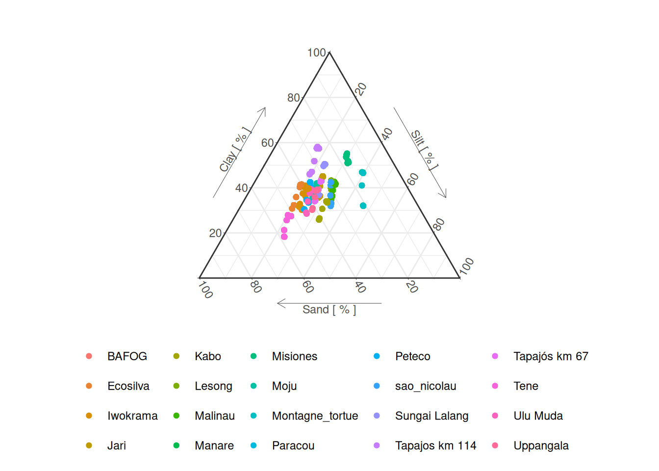
read_tsv("data/derived_data/soil.tsv") %>%
  ggplot(aes(x = sand, y = clay, z = silt, col = site)) +
  ggtern::coord_tern(L = "x", T = "y", R = "z") +
  geom_point() +
  theme_bw() +
  labs(
    yarrow = "Clay [ % ]",
    zarrow = "Silt [ % ]",
    xarrow = "Sand [ % ]"
  ) +
  ggtern::theme_showarrows() +
  ggtern::theme_hidetitles() +
  ggtern::theme_clockwise() +
  scale_color_discrete("") +
  theme(legend.position = "bottom", legend.key.size = unit(0.5, "line"))

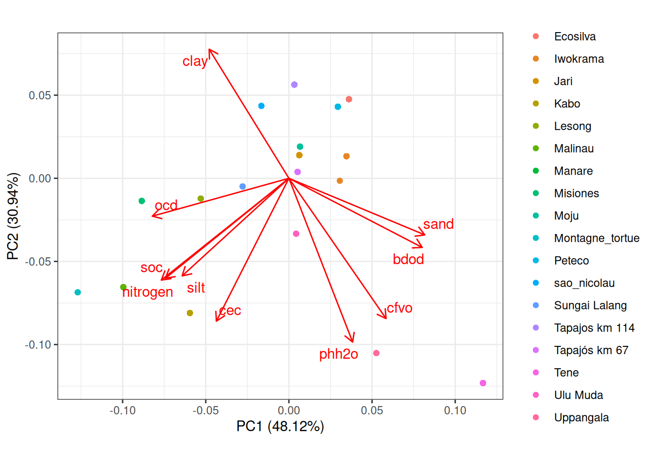
Soil texture for all sites, plots and depths.

The first ordination axis retained almost half of the variations of the 10 soil variables and opposed sandy poor soils to more fertile silty soils.

Code

library(ggfortify)
data <- read_tsv("data/derived_data/soil.tsv") %>%
  select(-X, -Y) %>%
  group_by(site) %>%
  filter(depth <= 15) %>%
  summarise_all(mean, na.omit = TRUE) %>%
  select(-ocs) %>%
  na.omit()
pca <- prcomp(data %>% select(-site, -depth), scale. = TRUE)
autoplot(pca,
  loadings = TRUE, loadings.label = TRUE,
  loadings.label.repel = TRUE,
  data = data, colour = "site"
) +
  theme_bw() +
  coord_equal() +
  scale_color_discrete("") +
  theme(legend.key.size = unit(0.5, "line"))

Code

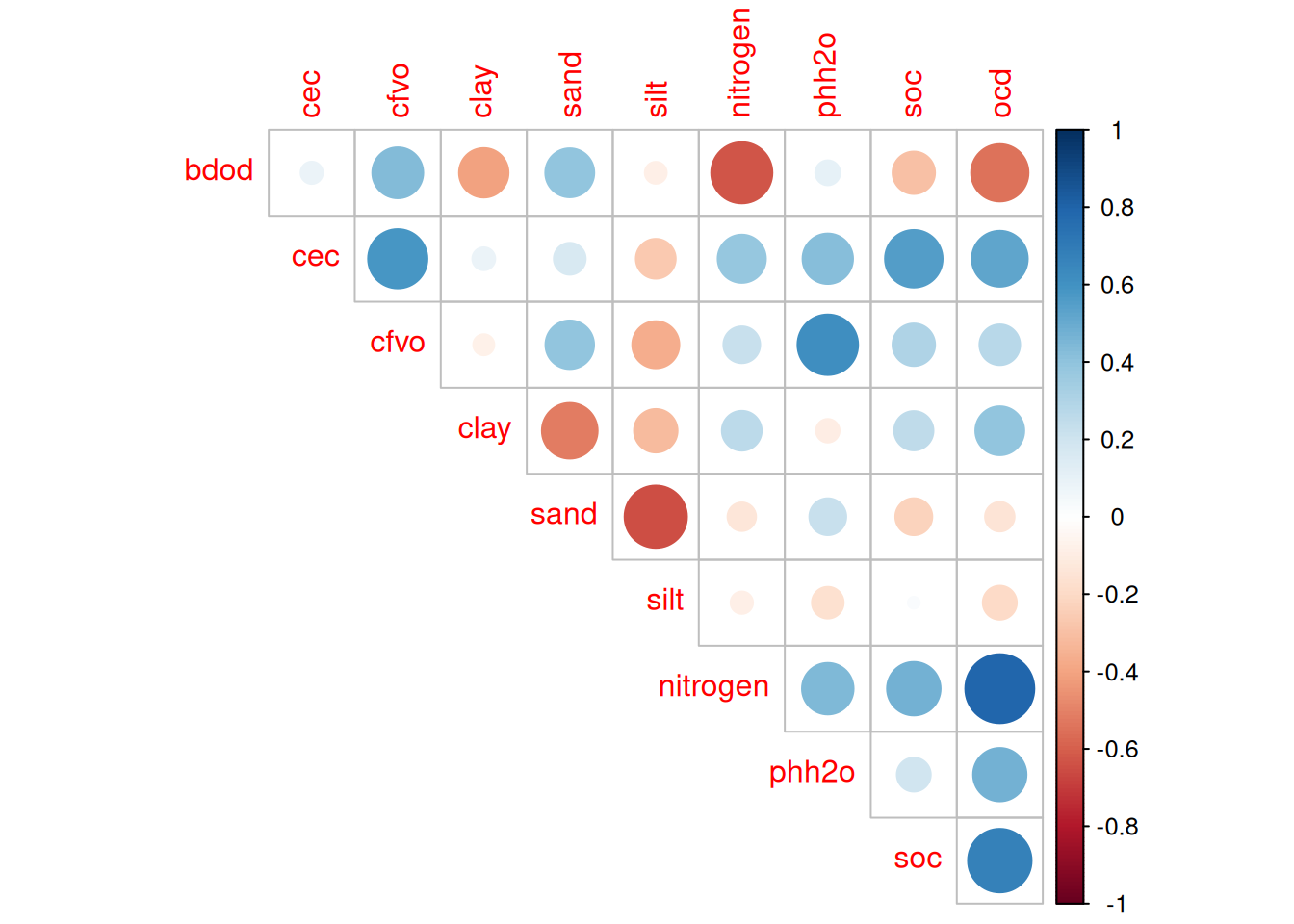
read_tsv("data/derived_data/soil.tsv") %>%
  select(-X, -Y) %>%
  group_by(site) %>%
  filter(depth <= 15) %>%
  summarise_all(mean, na.omit = TRUE) %>%
  select(-ocs) %>%
  na.omit() %>%
  select(-site, -depth) %>%
  cor(use = "pairwise.complete.obs") %>%
  corrplot::corrplot(type = "upper", diag = FALSE)

We will extract all for modelling but group 2 is focused on soil fertility with bulk density (bdod) and soil organic carbon (soc). Note that V. Freycon recommend using cay which is very linked to soil fertility in undistrubed tropical forests as well as to water properties.