For the moment we only used information on total forest cover area in a radius of 1-km from TMF (European Commission. Joint Research Centre. 2020). But the radius could be changed and other finer landscape indices could be derived and finer classification from TMF data could be used. Additionally, in landscape metrics WS1 metadata file listed also distance to the nearest village or road which could be simply extracted from openstreetmaps using R (osmdata).
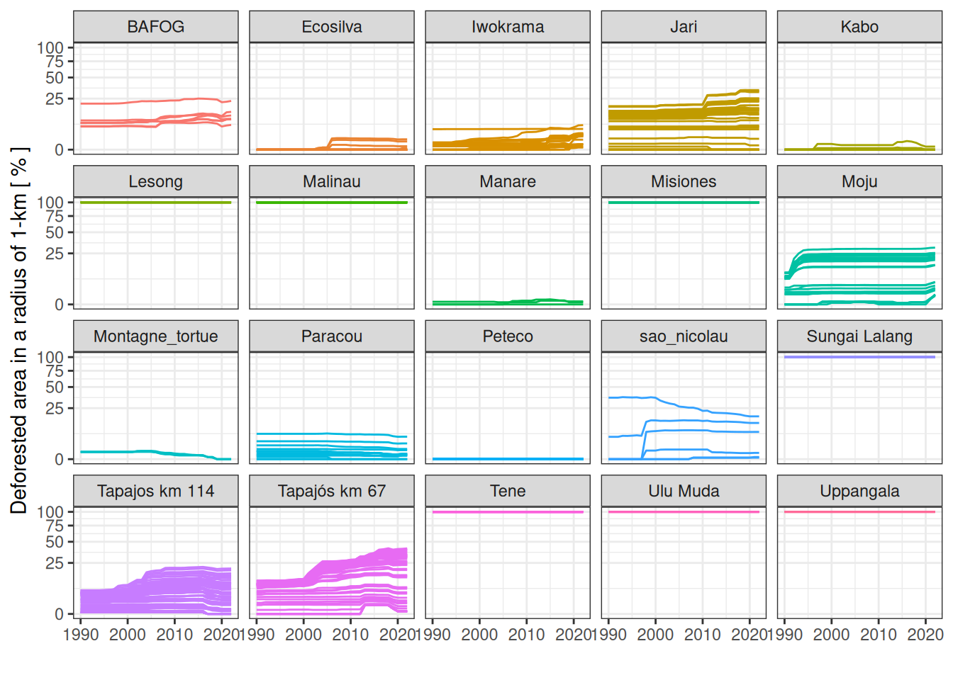
Most sites showed low deforestation level in the 90s but most of them showed deforestation increasing through time.
There are issues with locations of Lesong, Malinau, Missiones, Sungai Lalang, Tené, Ulu Muda, and Uppangala that doesn’t fall on forest according to TMF.
Code
read_tsv("outputs/landscape.tsv") %>%ggplot(aes(year, 100- intact, col = site, group =paste(site, plot))) +geom_line() +theme_bw() +xlab("") +ylab("Deforested area in a radius of 1-km [ % ]") +facet_wrap(~site) +scale_color_discrete(guide ="none") +scale_y_sqrt()
Forest cover through time.
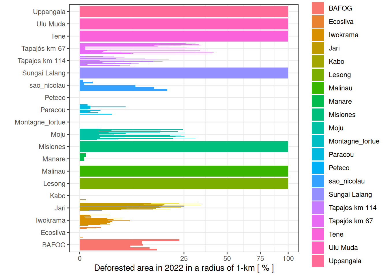
Most sites showed less than 10% forest loss cover in 2022, but few sites such as Tapajos km67 lost more than a third of their forest cover.
Code
read_tsv("outputs/landscape.tsv") %>%filter(year ==2022) %>%ggplot(aes(site, 100- intact, fill = site, group =paste(site, plot))) +geom_col(position ="dodge") +theme_bw() +xlab("") +ylab("Deforested area in 2022 in a radius of 1-km [ % ]") +scale_fill_discrete(" ") +coord_flip() +scale_y_sqrt()
2022 forest cover.
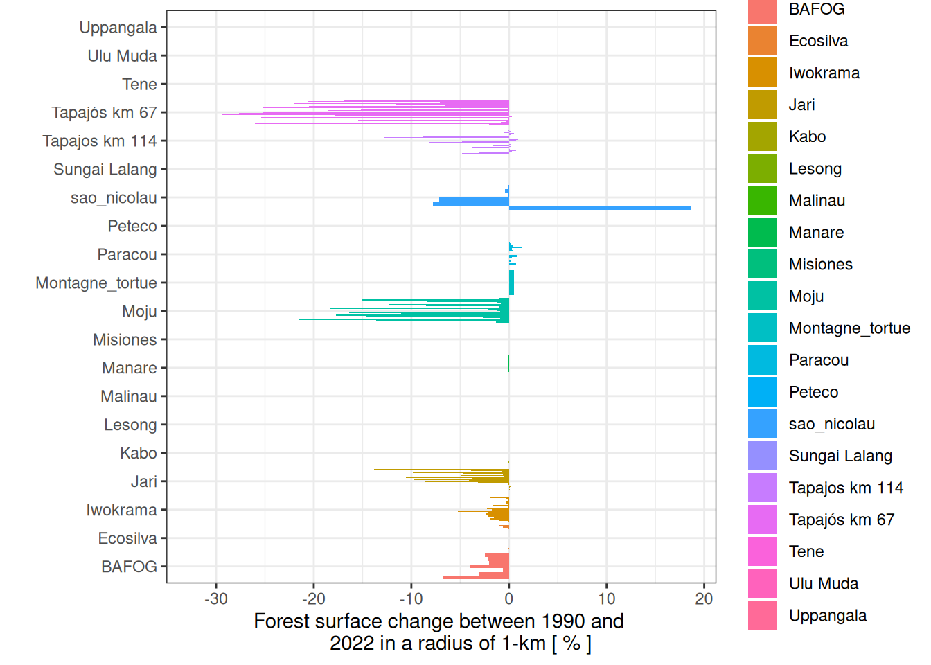
Almost all sites lost forest cover between 1990 and 2022 at the exception of few plots in Sao Nicolau that gained almost 20% of cover.
Code
read_tsv("outputs/landscape.tsv") %>%filter(year %in%c(1990, 2022)) %>%arrange(site, plot, year) %>%group_by(site, plot) %>%mutate(delta = intact -lag(intact)) %>%na.omit() %>%ggplot(aes(site, delta, fill = site, group =paste(site, plot))) +geom_col(position ="dodge") +theme_bw() +xlab("") +ylab("Forest surface change between 1990 and 2022 in a radius of 1-km [ % ]") +scale_fill_discrete(" ") +coord_flip()
Forest cover change between 1990 and 2022.
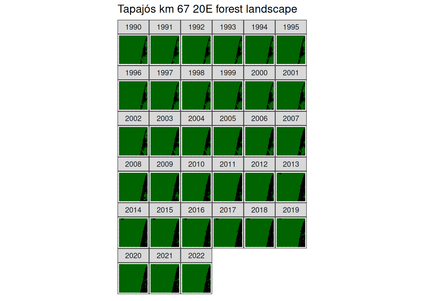
For each site we can use the intermediary files to project forest loss through time and derive finer landscape metrics if needed.
Code
read_tsv("data/derived_data/landscape/Tapajós km 67_20E_landscape.tsv") %>%ggplot(aes(lon, lat, fill =as.factor(forest))) +geom_raster() +facet_wrap(~year) +theme_bw() +coord_equal() +scale_fill_manual(guide ="none", values =c("black", "darkgreen")) +theme(axis.text =element_blank(),axis.title =element_blank(),axis.ticks =element_blank(),panel.spacing =unit(0, "lines") ) +ggtitle("Tapajós km 67 20E forest landscape")
Tapajós km 67 20E forest cover through time.
European Commission. Joint Research Centre. 2020. Long-term monitoring of tropical moist forest extent (from 1990 to 2019): description of the dataset. LU: Publications Office. https://doi.org/10.2760/70243.