Data
Code
plot_info <- read.csv("data/raw_data/bioforest-plot-information.csv") |>
  select(site, plot, Year_of_harvest, Treatment)
data <- read.csv("data/derived_data/aggregated_data_v9.csv") |>
  mutate(plot_new = Plot) |>
  separate(Plot, "Plot", "_") |>
  left_join(plot_info, by = join_by(Site == site, Plot == plot)) |>
  filter(grepl("cwmdiff", variable)) |>
  separate(variable, c("trait", NA, "flux"), sep = "_")
For now, we only calibrate the model with sites that have censuses every one to two years (Paracou, Mbaiki and SUAS).
Code
data <- data |>
  filter(Site %in% c("Paracou", "Mbaiki", "SUAS"))
Model
Code
data_rec <- data |>
  mutate(trec = Year - Year_of_harvest) |>
  filter(Treatment == "Logging" & trec > 3) |>
  filter(Site == "Paracou" & trait == "WD" & flux == "all") |>
  mutate(plotnum = as.numeric(as.factor(paste(Site, plot_new))))
mdata_cwd <- list(
  N = nrow(data_rec),
  K = 2,
  P = max(data_rec$plotnum),
  y = data_rec$value,
  plot = data_rec$plotnum,
  time = data_rec$trec
)
sample_model("exp_spline", mdata_cwd)
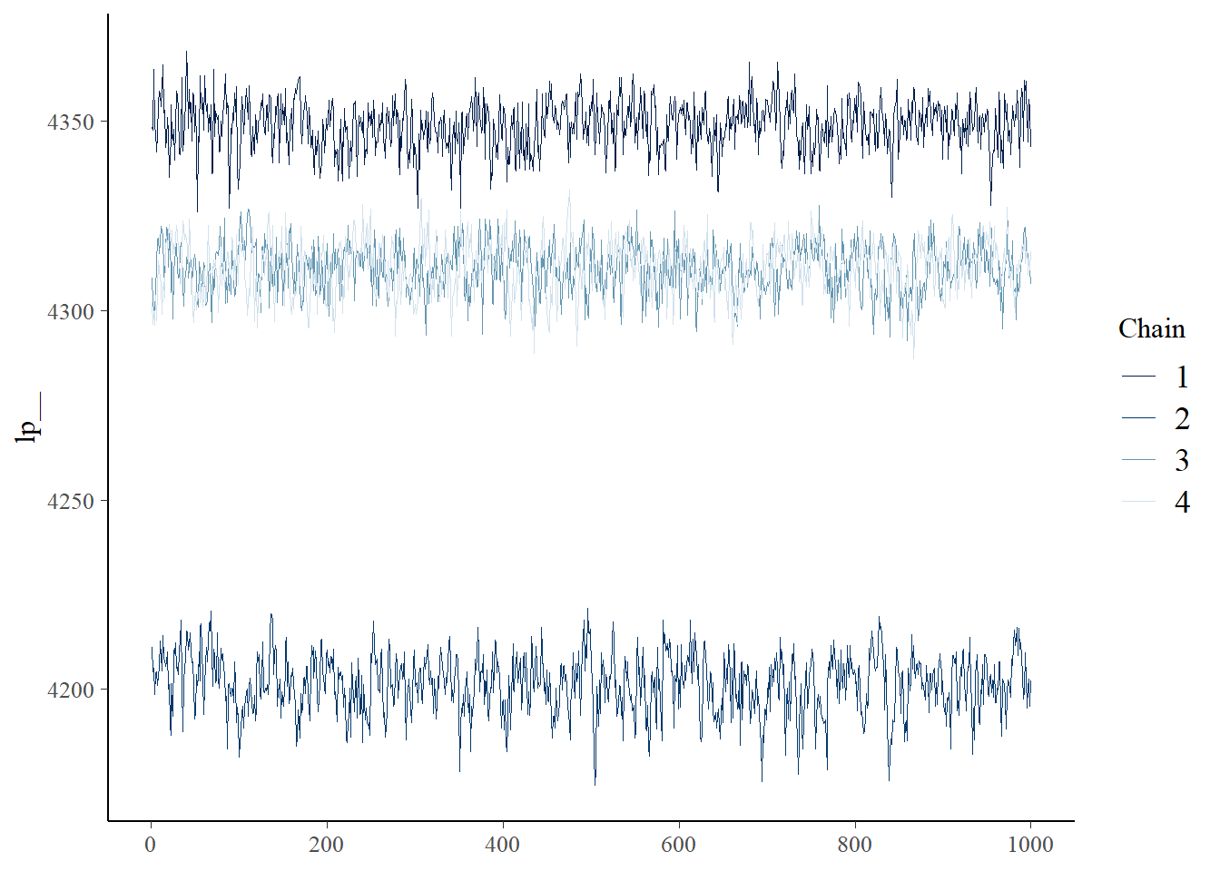
The resulting Stan fit summary is presented below.
Code
fit_flux_cwd <- as_cmdstan_fit(
  list.files("chains/exp_spline/", full.names = TRUE)
)
fit_flux_cwd
   variable    mean  median    sd   mad      q5     q95 rhat ess_bulk ess_tail
 lp__       4293.25 4311.71 55.60 28.55 4194.96 4354.45 2.41        4       30
 sigma         0.00    0.00  0.00  0.00    0.00    0.00 2.32        4       31
 dlogtau[1]    2.06    2.15  0.22  0.08    1.67    2.26 1.98        5       33
 dlogtau[2]    2.57    2.53  0.56  0.62    1.79    3.40 2.42        4       29
 nu[1]         1.25    0.88  0.96  0.54    0.38    2.95 2.10        5       33
 nu[2]         3.34    2.96  0.89  0.42    2.52    4.97 2.15        5       33
 delta[1,1]   -0.01   -0.01  0.00  0.00   -0.01    0.00 1.37        8       28
 delta[2,1]   -0.01   -0.01  0.00  0.00   -0.01   -0.01 1.05       53       67
 delta[3,1]    0.00    0.00  0.00  0.00    0.00    0.00 1.43        8       29
 delta[4,1]    0.00    0.00  0.00  0.00    0.00    0.00 1.37        8       29

 # showing 10 of 2135 rows (change via 'max_rows' argument or 'cmdstanr_max_rows' option)
Code
mcmc_trace(fit_flux_cwd$draws(variables = c("lp__")))
Code
c("tau", "delta", "nu") |>
  fit_flux_cwd$summary()
# A tibble: 76 × 10
   variable       mean   median      sd     mad       q5      q95  rhat ess_bulk
   <chr>         <dbl>    <dbl>   <dbl>   <dbl>    <dbl>    <dbl> <dbl>    <dbl>
 1 tau[1]      7.99     8.59    1.55e+0 7.23e-1  5.33     9.57e+0  1.98     5.52
 2 tau[2]     23.2     21.7     9.56e+0 8.38e+0 11.4      3.84e+1  2.42     4.90
 3 delta[1,1] -0.00663 -0.00681 1.23e-3 1.04e-3 -0.00838 -4.21e-3  1.37     8.82
 4 delta[2,1] -0.00652 -0.00647 9.16e-4 8.48e-4 -0.00814 -5.12e-3  1.05    53.4
 5 delta[3,1] -0.00284 -0.00307 1.31e-3 1.09e-3 -0.00463 -1.95e-4  1.43     8.09
 6 delta[4,1] -0.00194 -0.00215 1.25e-3 1.03e-3 -0.00367  5.18e-4  1.37     8.76
 7 delta[5,1] -0.00524 -0.00561 1.47e-3 1.11e-3 -0.00707 -2.25e-3  1.50     7.43
 8 delta[6,1] -0.00236 -0.00235 8.60e-4 7.86e-4 -0.00376 -9.57e-4  1.03   116.
 9 delta[7,1] -0.00571 -0.00589 1.22e-3 1.01e-3 -0.00740 -3.30e-3  1.36     9.09
10 delta[8,1] -0.00446 -0.00462 1.16e-3 9.78e-4 -0.00604 -2.17e-3  1.27    11.1
# ℹ 66 more rows
# ℹ 1 more variable: ess_tail <dbl>
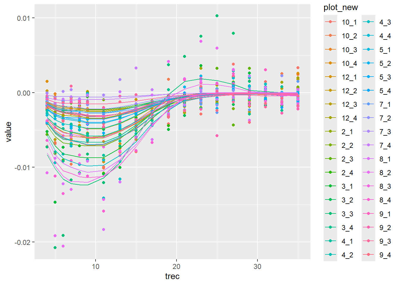
Code
data |>
  mutate(trec = Year - Year_of_harvest) |>
  filter(Treatment == "Logging" & trec > 3) |>
  filter(Site == "Paracou" & trait == "WD" & flux == "all") |>
  mutate(med =  fit_flux_cwd$summary("mu")$median) |>
  mutate(q5 =  fit_flux_cwd$summary("mu")$q5) |>
  mutate(q95 =  fit_flux_cwd$summary("mu")$q95) |>
  ggplot(aes(trec, value, col=plot_new)) +
  geom_point() +
  geom_line(aes(y=med))