Exploration of summary statistics

Code

environ <- readr::read_tsv("data/raw_data/environment.tsv")
params <- read_csv("data/derived_data/params_flux_all.csv")

site_info <- read.csv("data/derived_data/sites_to_keep.csv") %>%
  filter(ncensus >= 10) %>%
  mutate(
    continent =
      case_when(
        Site %in% c("Corinto", "Paracou", "Tapajos Km67")
        ~ "America",
        Site %in% c("Lesong", "SUAS", "Sungai Lalang", "Ulu Muda")
        ~ "Asia",
        Site %in% c("Mbaiki")
        ~ "Africa"
      )
  ) %>%
  left_join(environ, by = c("Site" = "site"))

plot_info_raw <- read.csv("data/raw_data/bioforest-plot-information.csv") %>%
  select(site, plot, Year_of_harvest, Treatment)

plot_info <- read_csv("data/derived_data/aggregated_data_v9.csv") %>%
  filter(Site %in% site_info$Site & variable %in% c("ba", "agb")) %>%
  mutate(plot_new = Plot) %>%
  separate(Plot, "Plot", "_") %>%
  pivot_wider(
    names_from = "variable",
    values_from = "value"
  ) %>%
  left_join(plot_info_raw, by = join_by(Site == site, Plot == plot)) %>%
  group_by(Site, plot_new, Treatment, Year_of_harvest) %>%
  summarise(
    census1 = min(Year),
    ba_0 = ba[Year == min(Year)],
    ba_min = min(ba[Year > Year_of_harvest &
                      Year <= Year_of_harvest + 5]),
    agb_0 = agb[Year == min(Year)]
  ) %>%
  mutate(
    ba_0 = if_else(census1 < Year_of_harvest, ba_0, NA),
    agb_0 = if_else(census1 < Year_of_harvest, agb_0, NA),
    intensity = (ba_0 - ba_min) / ba_0
  )


data_explo <- params %>%
  left_join(site_info) %>%
  left_join(plot_info)

Duration of over-mortality

We expect over-mortality to be due to the delayed mortality of damaged trees and to gap contagion (due to increased mortality at the edge of the gaps).

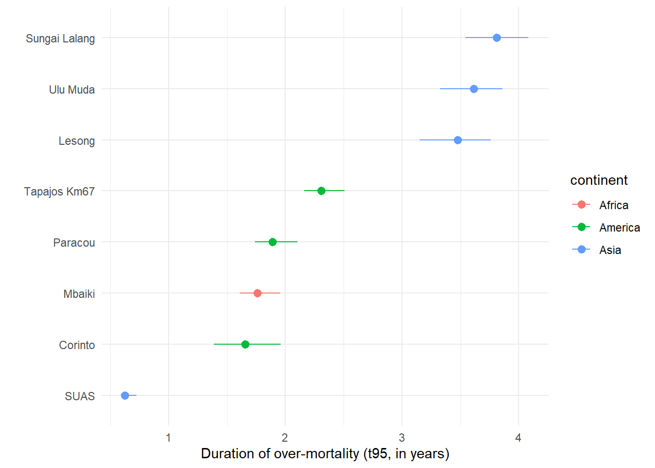
We expect it to occur within the first few years after logging => confirmed, over-mortality ends after less than 5 years.

Code

data_explo %>%
  filter(variable == "t95_m") %>%
  ggplot(aes(median, reorder(Site, median), col = continent)) +
  geom_pointrange(aes(xmin = q5, xmax = q95)) +
  labs(
    x = "Duration of over-mortality (t95, in years)",
    y = ""
  ) +
  theme_minimal()

We expect it to be quite consistent between sites => not confirmed, the sites have quite different duration of over-mortality. This is not due to the timing of the censuses after logging (trec):

Code

read_csv("data/derived_data/aggregated_data_v9.csv") %>%
  filter(Site %in% site_info$Site & variable == "ba") %>%
  mutate(plot_new = Plot) %>%
  separate(Plot, "Plot", "_") %>%
  left_join(plot_info) %>%
  mutate(trec = Year - Year_of_harvest) %>%
  filter(trec > 0 & trec < 6) %>%
  group_by(Site) %>%
  summarise(trec = paste(unique(trec), collapse = ", ")) %>%
  kable()

Site	trec
Corinto	1, 2, 3, 4, 5
Lesong	1, 2, 3, 4, 5
Mbaiki	1, 2, 3, 4, 5
Paracou	1, 2, 3, 4, 5
SUAS	2, 4
Sungai Lalang	1, 2, 3, 4, 5
Tapajos Km67	1, 2, 3, 4
Ulu Muda	1, 2, 3, 4, 5

The variability of timing is probably due to post-logging silvicultural treatment, but we cannot test this as the duration of over-mortality is estimated at the site level.

Duration of over-productivity

Over-productivity is due to the opening of the canopy cover that increases the growth of trees that are remnants from the logging, and allows the arrival and growth of new early successional individuals.

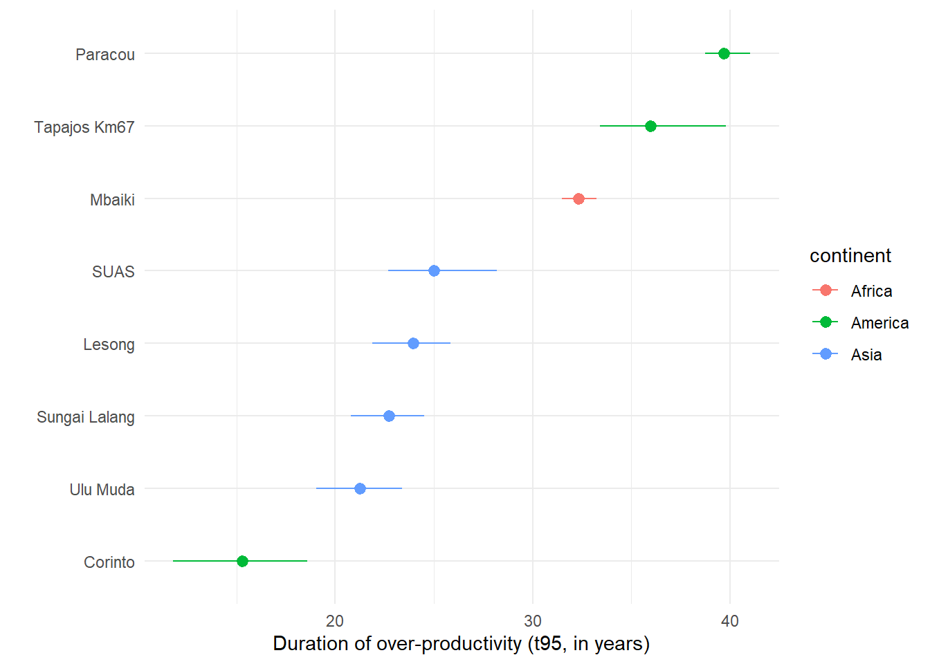
We expect it to last several decades as post-logging canopy closure takes several decades => confirmed.

Code

data_explo %>%
  filter(variable == "t95_p") %>%
  ggplot(aes(median, reorder(Site, median), col = continent)) +
  geom_pointrange(aes(xmin = q5, xmax = q95)) +
  labs(
    x = "Duration of over-productivity (t95, in years)",
    y = ""
  ) +
  theme_minimal()

We expect the variability of the duration of over-productivity to depends on:

the logging intensity => cannot be tested as this duration is fitted at the site scale
the ecology of the pioneer species (life span) => could that explain the effect of continent that seems to be quite clear, except for Corinto?
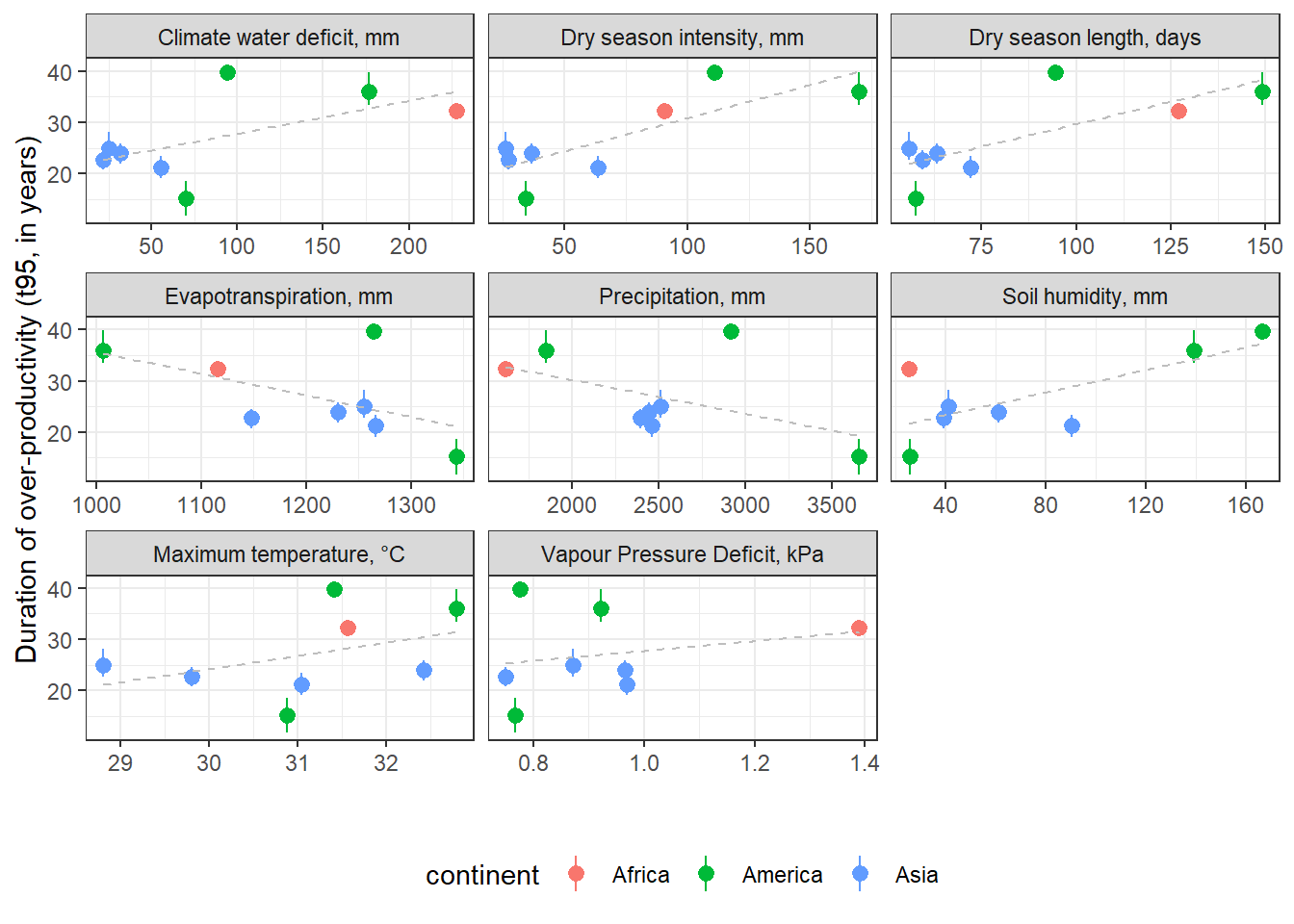
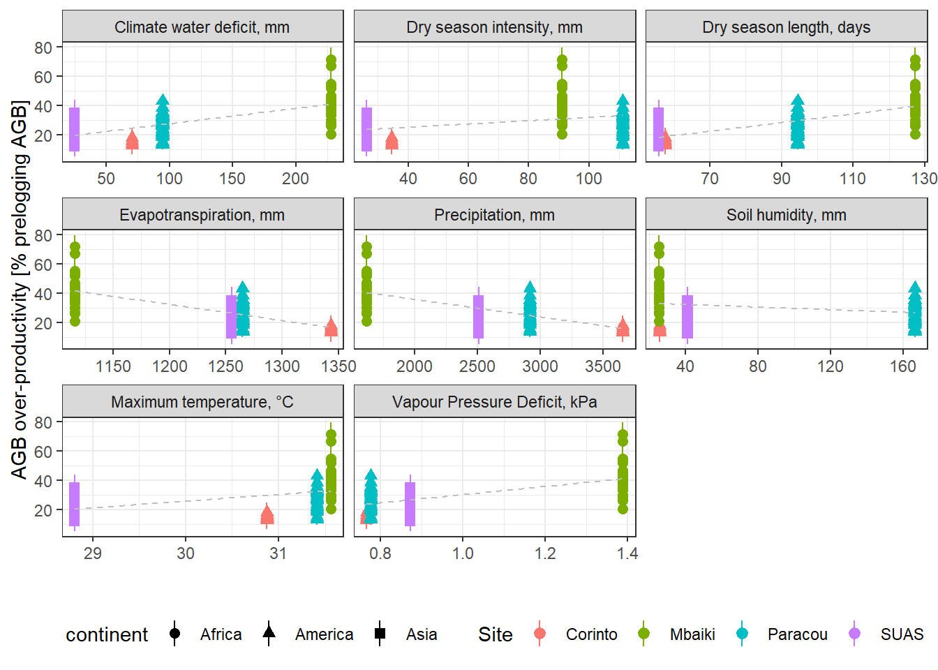
cimatic variables related to productivity => we see below that over-productivity has a longer duration in the drier sites (higher climate water deficit, dry season intensity and length, vapour pressure deficit (but this is driven by one outlier site) and lower evapotranspiration and precipitation). The pattern with soil humidity is however counter-intuitive (but soil humidity is very positively correlated with maximum temperature).

Code

data_explo %>%
  filter(variable == "t95_p") %>%
  select(
    Site, median, q5, q95,
    continent,
    et, cwd, pr, tmax, vpd, soil, dsl, dsi
  ) %>%
  pivot_longer(et:dsi, names_to = "var_clim", values_to = "value") %>%
  mutate(var_clim = fct_recode(var_clim,
    "Evapotranspiration, mm" = "et",
    "Climate water deficit, mm" = "cwd",
    "Precipitation, mm" = "pr",
    "Maximum temperature, °C" = "tmax",
    "Vapour Pressure Deficit, kPa" = "vpd",
    "Soil humidity, mm" = "soil",
    "Dry season length, days" = "dsl",
    "Dry season intensity, mm" = "dsi"
  )) %>%
  ggplot(aes(x = value, y = median)) +
  geom_pointrange(aes(ymin = q5, ymax = q95, col = continent)) +
  geom_smooth(
    method = "lm", se = FALSE,
    size = 0.5, col = "grey", linetype = "dashed"
  ) +
  labs(
    x = "",
    y = "Duration of over-productivity (t95, in years)"
  ) +
  facet_wrap(~var_clim, scales = "free_x") +
  theme_bw() +
  theme(legend.position = "bottom")

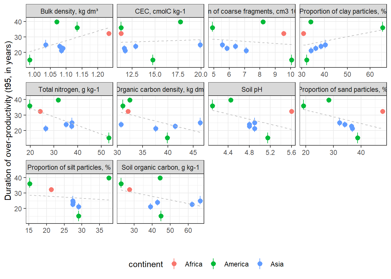
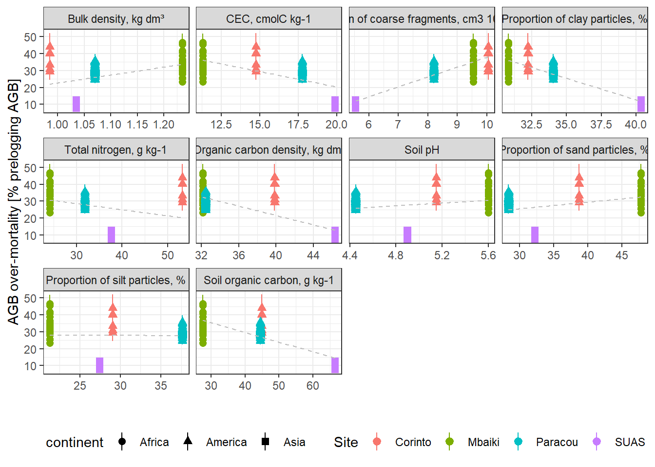
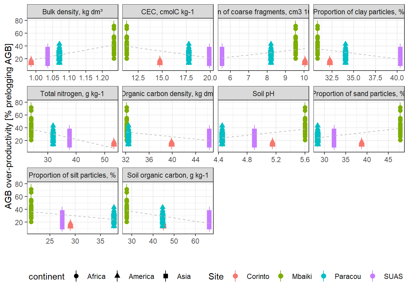
soil variables related to productivity => we see below that higher bulk density and lower SOC soils are related to longer duration of over-productivity, which would support the hypotheses that over-productivity lasts longer in less fertile soils. But the pattern obtained for clay content shows the opposite.

Code

data_explo %>%
  filter(variable == "t95_p") %>%
  select(
    Site, median, q5, q95,
    continent,
    bdod, cec, cfvo, clay, sand, silt, nitrogen, phh2o, soc, ocd
  ) %>%
  pivot_longer(bdod:ocd, names_to = "var_soil", values_to = "value") %>%
  mutate(var_soil = fct_recode(var_soil,
    "Bulk density, kg dm³" = "bdod",
    "CEC, cmolC kg-1" = "cec",
    "Fraction of coarse fragments, cm3 100cm-3" = "cfvo",
    "Proportion of clay particles, %" = "clay",
    "Proportion of sand particles, %" = "sand",
    "Proportion of silt particles, %" = "silt",
    "Total nitrogen, g kg-1" = "nitrogen",
    "Soil pH" = "phh2o",
    "Soil organic carbon, g kg-1" = "soc",
    "Organic carbon density, kg dm³" = "ocd"
  )) %>%
  ggplot(aes(x = value, y = median)) +
  geom_pointrange(aes(ymin = q5, ymax = q95, col = continent)) +
  geom_smooth(
    method = "lm", se = FALSE,
    size = 0.5, col = "grey", linetype = "dashed"
  ) +
  labs(
    x = "",
    y = "Duration of over-productivity (t95, in years)"
  ) +
  facet_wrap(~var_soil, scales = "free_x") +
  theme_bw() +
  theme(legend.position = "bottom")

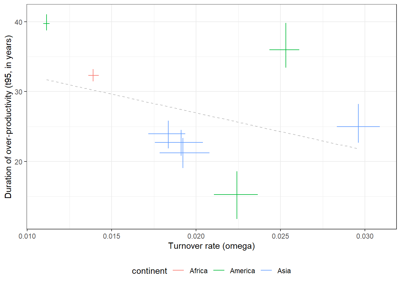
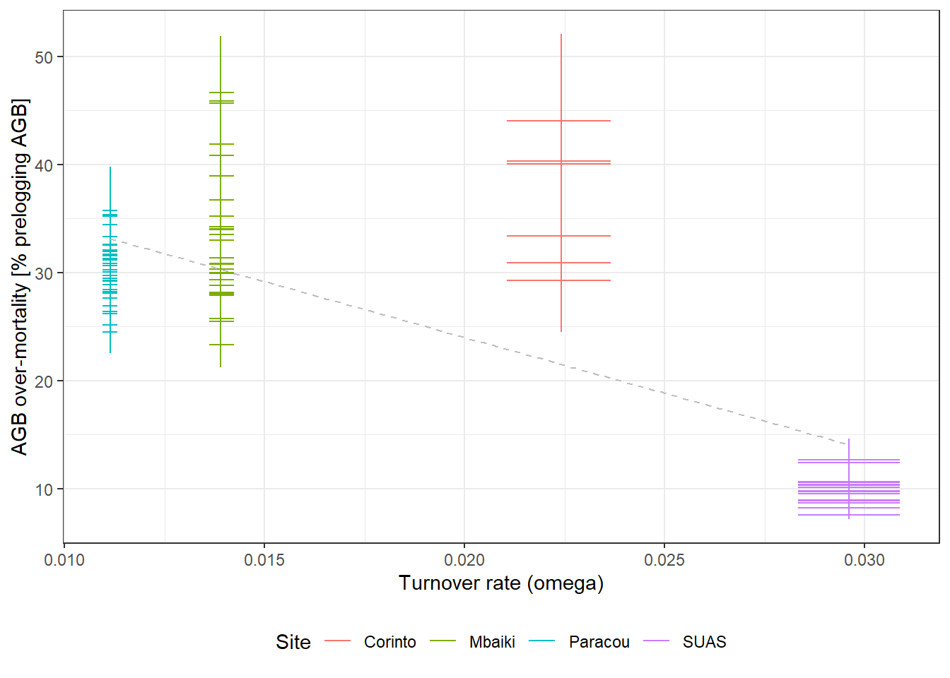
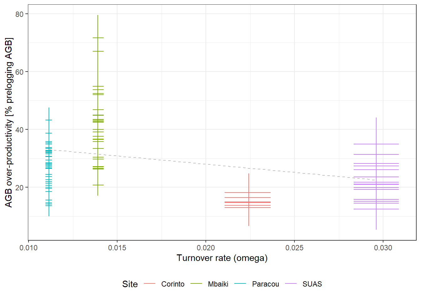
forest dynamism (turnover rate) => we see below that more dynamic sites (higher turnover rate \(\omega\)) have a lower duration of over-productivity.

Code

data_explo %>%
  filter(variable %in% c("omega", "t95_p")) %>%
  select(Site, variable, median, q5, q95, continent) %>%
  pivot_wider(
    names_from = variable,
    values_from = c(median, q5, q95)
  ) %>%
  ggplot(aes(x = median_omega, y = median_t95_p)) +
  geom_errorbar(aes(
    ymin = q5_t95_p, ymax = q95_t95_p,
    col = continent,
    width = 0
  )) +
  geom_errorbarh(aes(
    xmin = q5_omega, xmax = q95_omega,
    col = continent,
    height = 0
  )) +
  geom_smooth(
    method = "lm", se = FALSE,
    size = 0.5, col = "grey", linetype = "dashed"
  ) +
  labs(
    x = "Turnover rate (omega)",
    y = "Duration of over-productivity (t95, in years)"
  ) +
  theme_bw() +
  theme(legend.position = "bottom")

The trends observed seems to generally support the hypothesis that over-productivity would lask longuer is less productive (drier and less fertile) and less dynamic sites (lower turnover rate), which would make sense. Let’s be careful not to over interpret it though, as there are just 8 sites and possible confunding effects due to the correlation among environmental factors in the data set.

Relative over-mortality

We consider relative over-mortality, being the AGB of total over-mortality expressed as a percentage of pre-logging AGB. For this, we need pre-logging censuses, which are not available for the site of Lesong, Sungai Lalang, Tapajos and Ulu Muda. This analyis is therefore limited to 4 sites for the time being.

We could consider another way to standardise over-mortality, for exemple by using the stock estimated at infinite time by the model (but we first need to check how well it matches pre-logging AGB), or by considering the AGB of control plots (but we first need to check how much intrasite variability the is).

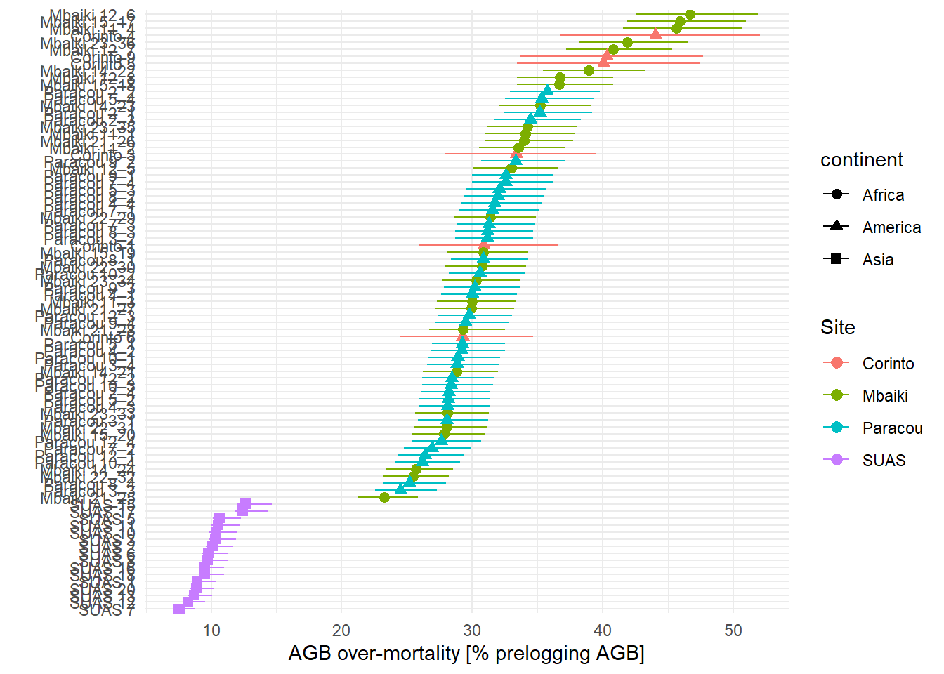
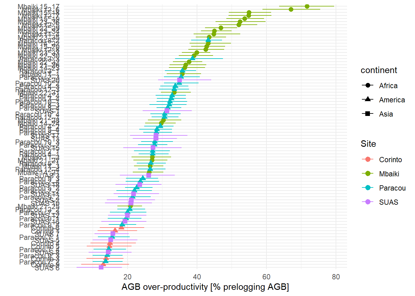
The graph below show that there is a lot of variability in the relative AGB over-mortality, with values going from less than 30% to almost 80%.

80% is very high, to check…

Code

data_explo %>%
  filter(variable == "int_m" & !(is.na(agb_0))) %>%
  mutate(site_plot = paste(Site, plot_new)) %>%
  ggplot(aes(median * 100 / agb_0,
    reorder(site_plot, median * 100 / agb_0),
    col = Site,
    shape = continent
  )) +
  geom_pointrange(aes(
    xmin = q5 * 100 / agb_0,
    xmax = q95 * 100 / agb_0
  )) +
  labs(
    x = "AGB over-mortality [% prelogging AGB]",
    y = ""
  ) +
  theme_minimal()

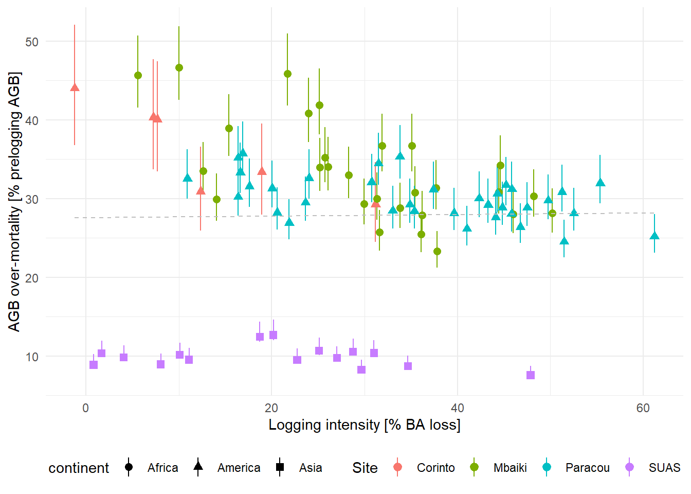
We expect that this variability would be partly explained by logging intensity, with a higher over-mortality when logging intensity is higher => this is not confirmed, as the graph below shows the opposite. There seems to be a strong site effect, but the within site trends seems to show that relative-overmortality decreases with logging intensity as well.

Code

data_explo %>%
  filter(variable == "int_m" & !(is.na(agb_0))) %>%
  mutate(Site = fct_drop(as.factor(Site))) %>%
  ggplot(aes(
    x = intensity * 100,
    y = median * 100 / agb_0
  )) +
  geom_pointrange(aes(
    ymin = q5 * 100 / agb_0,
    ymax = q95 * 100 / agb_0,
    col = Site,
    shape = continent
  )) +
  geom_smooth(
    method = "lm", se = FALSE,
    size = 0.5, col = "grey", linetype = "dashed"
  ) +
  labs(
    x = "Logging intensity [% BA loss]",
    y = "AGB over-mortality [% prelogging AGB]"
  ) +
  theme_minimal() +
  theme(legend.position = "bottom")

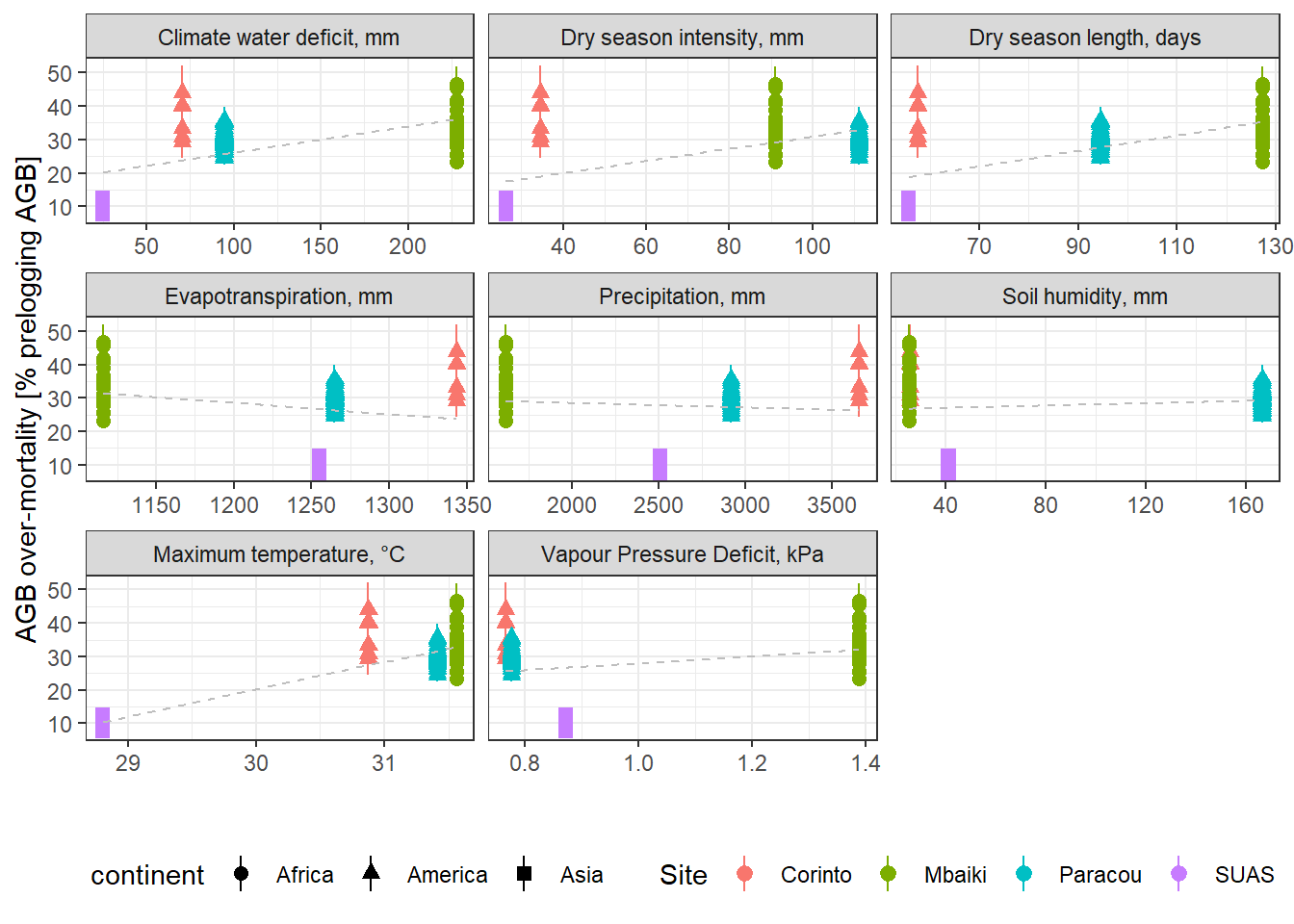
I have no real hypothesis on the effect of environmental variables on the relative over-mortality, but I make some graph anyway, in case some people have. NB: the environmental variables are available at the site level, so with 4 sites, I don’t think we will be able to say much.

Climate variables: the graphs below suggest that relative over-mortality is lower in drier sites.

Code

data_explo %>%
  filter(variable == "int_m" & !(is.na(agb_0))) %>%
  select(
    Site, plot_new, median, q5, q95, agb_0,
    continent,
    et, cwd, pr, tmax, vpd, soil, dsl, dsi
  ) %>%
  pivot_longer(et:dsi, names_to = "var_clim", values_to = "value") %>%
  mutate(var_clim = fct_recode(var_clim,
    "Evapotranspiration, mm" = "et",
    "Climate water deficit, mm" = "cwd",
    "Precipitation, mm" = "pr",
    "Maximum temperature, °C" = "tmax",
    "Vapour Pressure Deficit, kPa" = "vpd",
    "Soil humidity, mm" = "soil",
    "Dry season length, days" = "dsl",
    "Dry season intensity, mm" = "dsi"
  )) %>%
  ggplot(aes(x = value, y = median * 100 / agb_0)) +
  geom_pointrange(aes(
    ymin = q5 * 100 / agb_0,
    ymax = q95 * 100 / agb_0,
    col = Site,
    shape = continent
  )) +
  geom_smooth(
    method = "lm", se = FALSE,
    size = 0.5, col = "grey", linetype = "dashed"
  ) +
  labs(
    x = "",
    y = "AGB over-mortality [% prelogging AGB]"
  ) +
  facet_wrap(~var_clim, scales = "free_x") +
  theme_bw() +
  theme(legend.position = "bottom")

Soil variables: the graphs below suggest that relative over-mortality is lower in less fertile soils.

Code

data_explo %>%
  filter(variable == "int_m" & !(is.na(agb_0))) %>%
  select(
    Site, median, q5, q95, agb_0,
    continent,
    bdod, cec, cfvo, clay, sand, silt, nitrogen, phh2o, soc, ocd
  ) %>%
  pivot_longer(bdod:ocd, names_to = "var_soil", values_to = "value") %>%
  mutate(var_soil = fct_recode(var_soil,
    "Bulk density, kg dm³" = "bdod",
    "CEC, cmolC kg-1" = "cec",
    "Fraction of coarse fragments, cm3 100cm-3" = "cfvo",
    "Proportion of clay particles, %" = "clay",
    "Proportion of sand particles, %" = "sand",
    "Proportion of silt particles, %" = "silt",
    "Total nitrogen, g kg-1" = "nitrogen",
    "Soil pH" = "phh2o",
    "Soil organic carbon, g kg-1" = "soc",
    "Organic carbon density, kg dm³" = "ocd"
  )) %>%
  ggplot(aes(x = value, y = median * 100 / agb_0)) +
  geom_pointrange(aes(
    ymin = q5 * 100 / agb_0,
    ymax = q95 * 100 / agb_0,
    col = Site,
    shape = continent
  )) +
  geom_smooth(
    method = "lm", se = FALSE,
    size = 0.5, col = "grey", linetype = "dashed"
  ) +
  labs(
    x = "",
    y = "AGB over-mortality [% prelogging AGB]"
  ) +
  facet_wrap(~var_soil, scales = "free_x") +
  theme_bw() +
  theme(legend.position = "bottom")

Forest dynamism (turnover rate \(\omega\)): the graph below shows that over-mortality increases with turnover rate.

Code

dt_omega <- data_explo %>%
  filter(variable == "omega") %>%
  select(Site, median, q5, q95) %>%
  rename(
    median_omega = median,
    q5_omega = q5,
    q95_omega = q95
  )

data_explo %>%
  filter(variable == "int_m" & !(is.na(agb_0))) %>%
  select(Site, variable, median, q5, q95, agb_0, continent) %>%
  left_join(dt_omega) %>%
  ggplot(aes(x = median_omega, y = median * 100 / agb_0)) +
  geom_errorbar(
    aes(
      ymin = q5 * 100 / agb_0,
      ymax = q95 * 100 / agb_0,
      col = Site,
      shape = continent
    ),
    width = 0
  ) +
  geom_errorbarh(
    aes(
      xmin = q5_omega,
      xmax = q95_omega,
      col = Site,
      shape = continent
    ),
    height = 0
  ) +
  geom_smooth(
    method = "lm", se = FALSE,
    size = 0.5, col = "grey", linetype = "dashed"
  ) +
  labs(
    x = "Turnover rate (omega)",
    y = "AGB over-mortality [% prelogging AGB]"
  ) +
  theme_bw() +
  theme(legend.position = "bottom")

Relative over-productivity

We consider relative over-productivity, being the AGB of total over-productivity expressed as a percentage of pre-logging AGB. For this, we need pre-logging censuses, which are not available for the site of Lesong, Sungai Lalang, Tapajos and Ulu Muda. This analyis is therefore limited to 4 sites for the time being.

We could consider another way to standardise over-productivity, for exemple by using the stock estimated at infinite time by the model (but we first need to check how well it matches pre-logging AGB), or by considering the AGB of control plots (but we first need to check how much intrasite variability the is).

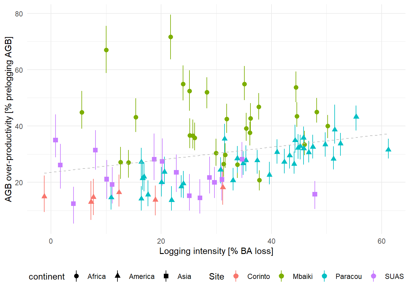
The graph below show that there is a lot of variability in the relative AGB over-mortality, with values going from less than 10% to almost 80%*.

Code

data_explo %>%
  filter(variable == "int_p" & !(is.na(agb_0))) %>%
  mutate(site_plot = paste(Site, plot_new)) %>%
  ggplot(aes(median * 100 / agb_0,
    reorder(site_plot, median * 100 / agb_0),
    col = Site,
    shape = continent
  )) +
  geom_pointrange(aes(
    xmin = q5 * 100 / agb_0,
    xmax = q95 * 100 / agb_0
  )) +
  labs(
    x = "AGB over-productivity [% prelogging AGB]",
    y = ""
  ) +
  theme_minimal()

We expect that this variability would be partly explained by logging intensity, with a higher over-productivity when logging intensity is higher => this is confirmed by the graph below (but see the Mbaiki plots).

Code

data_explo %>%
  filter(variable == "int_p" & !(is.na(agb_0))) %>%
  mutate(Site = fct_drop(as.factor(Site))) %>%
  ggplot(aes(
    x = intensity * 100,
    y = median * 100 / agb_0
  )) +
  geom_pointrange(aes(
    ymin = q5 * 100 / agb_0,
    ymax = q95 * 100 / agb_0,
    col = Site,
    shape = continent
  )) +
  geom_smooth(
    method = "lm", se = FALSE,
    size = 0.5, col = "grey", linetype = "dashed"
  ) +
  labs(
    x = "Logging intensity [% BA loss]",
    y = "AGB over-productivity [% prelogging AGB]"
  ) +
  theme_minimal() +
  theme(legend.position = "bottom")

I have no real hypothesis on the effect of environmental variables on the relative over-productivity, but I make some graphs anyway, in case some people have. NB: the environmental variables are available at the site level, so with 4 sites, I don’t think we will be able to say much.

Climate variables: the graphs below suggest that relative over-productivity is higher in drier sites.

Code

data_explo %>%
  filter(variable == "int_p" & !(is.na(agb_0))) %>%
  select(
    Site, plot_new, median, q5, q95, agb_0,
    continent,
    et, cwd, pr, tmax, vpd, soil, dsl, dsi
  ) %>%
  pivot_longer(et:dsi, names_to = "var_clim", values_to = "value") %>%
  mutate(var_clim = fct_recode(var_clim,
    "Evapotranspiration, mm" = "et",
    "Climate water deficit, mm" = "cwd",
    "Precipitation, mm" = "pr",
    "Maximum temperature, °C" = "tmax",
    "Vapour Pressure Deficit, kPa" = "vpd",
    "Soil humidity, mm" = "soil",
    "Dry season length, days" = "dsl",
    "Dry season intensity, mm" = "dsi"
  )) %>%
  ggplot(aes(x = value, y = median * 100 / agb_0)) +
  geom_pointrange(aes(
    ymin = q5 * 100 / agb_0,
    ymax = q95 * 100 / agb_0,
    col = Site,
    shape = continent
  )) +
  geom_smooth(
    method = "lm", se = FALSE,
    size = 0.5, col = "grey", linetype = "dashed"
  ) +
  labs(
    x = "",
    y = "AGB over-productivity [% prelogging AGB]"
  ) +
  facet_wrap(~var_clim, scales = "free_x") +
  theme_bw() +
  theme(legend.position = "bottom")

Soil variables: the graphs below suggest that relative over-productivity is higher in less fertile soils.

Code

data_explo %>%
  filter(variable == "int_p" & !(is.na(agb_0))) %>%
  select(
    Site, median, q5, q95, agb_0,
    continent,
    bdod, cec, cfvo, clay, sand, silt, nitrogen, phh2o, soc, ocd
  ) %>%
  pivot_longer(bdod:ocd, names_to = "var_soil", values_to = "value") %>%
  mutate(var_soil = fct_recode(var_soil,
    "Bulk density, kg dm³" = "bdod",
    "CEC, cmolC kg-1" = "cec",
    "Fraction of coarse fragments, cm3 100cm-3" = "cfvo",
    "Proportion of clay particles, %" = "clay",
    "Proportion of sand particles, %" = "sand",
    "Proportion of silt particles, %" = "silt",
    "Total nitrogen, g kg-1" = "nitrogen",
    "Soil pH" = "phh2o",
    "Soil organic carbon, g kg-1" = "soc",
    "Organic carbon density, kg dm³" = "ocd"
  )) %>%
  ggplot(aes(x = value, y = median * 100 / agb_0)) +
  geom_pointrange(aes(
    ymin = q5 * 100 / agb_0,
    ymax = q95 * 100 / agb_0,
    col = Site,
    shape = continent
  )) +
  geom_smooth(
    method = "lm", se = FALSE,
    size = 0.5, col = "grey", linetype = "dashed"
  ) +
  labs(
    x = "",
    y = "AGB over-productivity [% prelogging AGB]"
  ) +
  facet_wrap(~var_soil, scales = "free_x") +
  theme_bw() +
  theme(legend.position = "bottom")

Forest dynamism (turnover rate \(\omega\)): the graph below shows that over-mortality decreases with turnover rate.

Code

data_explo %>%
  filter(variable == "int_p" & !(is.na(agb_0))) %>%
  select(Site, variable, median, q5, q95, agb_0, continent) %>%
  left_join(dt_omega) %>%
  ggplot(aes(x = median_omega, y = median * 100 / agb_0)) +
  geom_errorbar(
    aes(
      ymin = q5 * 100 / agb_0,
      ymax = q95 * 100 / agb_0,
      col = Site,
      shape = continent
    ),
    width = 0
  ) +
  geom_errorbarh(
    aes(
      xmin = q5_omega,
      xmax = q95_omega,
      col = Site,
      shape = continent
    ),
    height = 0
  ) +
  geom_smooth(
    method = "lm", se = FALSE,
    size = 0.5, col = "grey", linetype = "dashed"
  ) +
  labs(
    x = "Turnover rate (omega)",
    y = "AGB over-productivity [% prelogging AGB]"
  ) +
  theme_bw() +
  theme(legend.position = "bottom")