Joint Genus

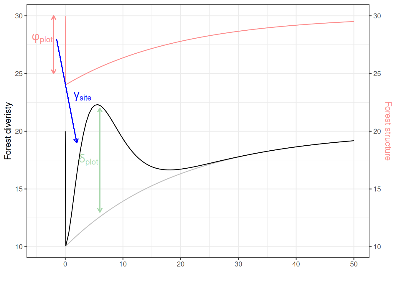
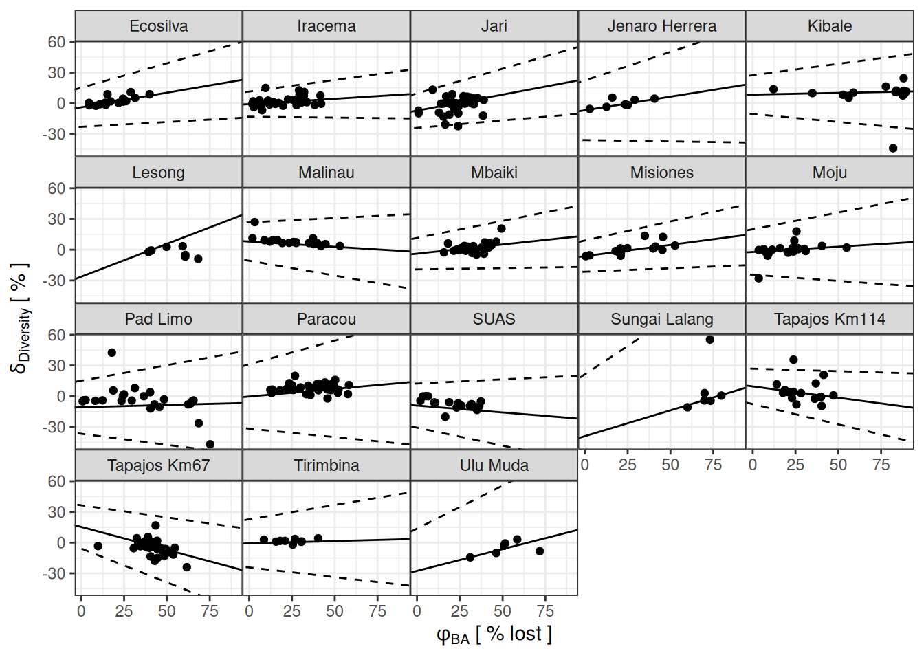
The model is the same as the modelling framework, but we want to establish a connection between the trajectory of forest structure, as represented by basal area, and forest diversity, as represented by genus diversity.

Equilibirum

Equilibrium model using control and pre-logging inventories to inform \(\theta\) prior of the recovery trajectory:

\[ \begin{align} BA \sim \mathcal N (\mu_{BA,site}+\delta_{BA,plot}, \sigma_{BA})\\ \delta_{BA,plot} \sim \mathcal N(0,\sigma_{BA,plot}) \\ y \sim \mathcal N (\mu_{site}+\delta_{plot}, \sigma)\\ \delta_{plot} \sim \mathcal N(0,\sigma_{plot}) \end{align} \]

Recovery

Recovery trajectory model:

\[ \begin{align} log(BA) \sim \mathcal N (log(\mu_{BA}), \sigma_{BA})\\ \mu_{BA} = \theta_{BA,site} \times (\phi_{BA,plot} + LTP_{BA} \times (1 - \phi_{plot}) + STP_{BA}) \\ LTP_{BA} = 1 - e^{-\lambda_{BA,plot} \times t} \\ STP_{BA} = \delta_{BA,plot} \times (\frac{t}{\tau_{BA,site}} \times e^{1-\frac{t}{\tau_{BA,site}}})^2 \\ log(y) \sim \mathcal N (log(\mu), \sigma)\\ \mu = \theta_{site} \times (\phi_{plot} + LTP \times (1 - \phi_{plot}) + STP) \\ LTP = 1 - e^{-\lambda_{plot} \times t} \\ STP = \delta_{plot} \times (\frac{t}{\tau_{site}} \times e^{1-\frac{t}{\tau_{site}}})^2 \\ \delta_{plot} \sim \mathcal N ( \delta0_{site}+\phi_{BA,plot} \times \gamma_{site}, \sigma_{\delta}) \end{align} \]

With the big novelty being:

\[ \delta_{plot} \sim \mathcal N ( \delta0_{site}+\phi_{BA,plot} \times \gamma_{site}, \sigma_{\delta}) \]

With the function linking the two to be defined.

Code

ltp <- function(time, dist, thetainf, lambda) {
  theta0 <- thetainf * dist
  ltp <- 1 - exp(-lambda * time)
  theta0 + (thetainf - theta0) * (ltp)
}
stp <- function(time, dist, thetainf, lambda, tau, delta) {
  theta0 <- thetainf * dist
  ltp <- 1 - exp(-lambda * time)
  stp <- delta * (time / tau * exp(1 - time / tau))^2
  theta0 + ltp * (thetainf - theta0) + stp * thetainf
}
data.frame(time = seq(0.1, 50, length.out = 100)) %>%
  mutate(y_ba = stp(time,
    dist = 0.8, thetainf = 30, lambda = 0.05,
    tau = 5, delta = 0
  )) %>% 
  mutate(y_stp = stp(time,
    dist = 0.5, thetainf = 20, lambda = 0.05,
    tau = 5, delta = 0.5
  )) %>%
  mutate(y_ltp = ltp(time, dist = 0.5, thetainf = 20, lambda = 0.05)) %>%
  bind_rows(data.frame(time = 0, y_stp = 20, y_ltp = 20, y_ba = 30)) %>%
  ggplot(aes(time)) +
  geom_line(aes(y = y_ba), col = "#fc8a8a") +
  geom_line(aes(y = y_ltp), col = "grey") +
  geom_line(aes(y = y_stp)) +
  theme_bw() +
  xlab("") + 
  scale_y_continuous(
    name = "Forest diveristy",
    sec.axis = sec_axis(~.*1, name = "Forest structure")
  ) +
  theme(
    axis.title.y.right = element_text(color = "#fc8a8a")
  ) +
  annotate("text",
    x = -4, y = 28, label = "phi[plot]",
    col = "#fc8a8a", parse = TRUE, size = 5
  ) +
    geom_segment(aes(x = -2, y = 25, xend = -2, yend = 30),
    arrow = arrow(length = unit(0.2, "cm")), col = "#fc8a8a"
  ) +
  geom_segment(aes(x = -2, y = 30, xend = -2, yend = 25),
    arrow = arrow(length = unit(0.2, "cm")), col = "#fc8a8a"
  ) +
  annotate("text",
    x = 4, y = 17.5, label = "delta[plot]",
    col = "#a7d6ac", parse = TRUE, size = 5
  ) +
  geom_segment(aes(x = 6, y = 13, xend = 6, yend = 22),
    arrow = arrow(length = unit(0.2, "cm")), col = "#a7d6ac"
  ) +
  geom_segment(aes(x = 6, y = 22, xend = 6, yend = 13),
    arrow = arrow(length = unit(0.2, "cm")), col = "#a7d6ac"
  ) +
  geom_segment(aes(x = -1.5, y = 28, xend = 2, yend = 19),
    arrow = arrow(length = unit(0.2, "cm")), col = "blue"
  ) +
  annotate("text",
    x = 3, y = 23, label = "gamma[site]",
    col = "blue", parse = TRUE, size = 5
  )

STP proj with pars.

Fit

Code

data <- read_tsv("../modelling/data/derived_data/data_rec.tsv", col_types = cols()) %>%
  select(-y) %>% 
  filter(variable %in% c("ba", "diversity_q1_gen")) %>%
  select(-sitenum, -plotnum) %>% 
  pivot_wider(names_from = variable, values_from = value) %>% 
  na.omit() %>% 
  filter(!(site %in% c("Manare", "Montagne Tortue", "Nelliyampathy",
                         "Uppangala", "BAFOG", "Sao Nicolau",
                         "Kabo", "Mil", "Corinto",
                         "Peixoto", "Iwokrama", "Antimary", "Peteco"))) %>% 
  mutate(sitenum = as.numeric(as.factor(site))) %>% 
  mutate(plotnum = as.numeric(as.factor(paste(site, plot)))) %>% 
  arrange(sitenum, plotnum, rel_year)  %>% 
  gather(variable, y, -plot, -year, -site, -treatment, -harvest_year,
         -longitude, -harvest_year_min, -rel_year, -sitenum, -plotnum)
trajectories <- read_tsv("chains/joint-diversity_q1_gen-trajectories.tsv")
parameters <-  read_tsv("chains/joint-diversity_q1_gen-parameters.tsv")
parameters

# A tibble: 727 × 14
   variable       mean   median      sd     mad       q5      q95  rhat ess_bulk
   <chr>         <dbl>    <dbl>   <dbl>   <dbl>    <dbl>    <dbl> <dbl>    <dbl>
 1 lp__     16799.      1.68e+4 108.    103.     1.66e+4  1.70e+4  1.97     5.52
 2 gamma       -0.285  -2.80e-1   0.191   0.182 -5.94e-1  2.88e-2  1.00  1551.  
 3 gamma       -0.104  -9.94e-2   0.123   0.122 -3.11e-1  8.83e-2  1.01   927.  
 4 gamma       -0.314  -3.19e-1   0.168   0.164 -5.81e-1 -3.06e-2  1.02   255.  
 5 gamma       -0.266  -2.55e-1   0.291   0.272 -7.45e-1  1.97e-1  1.00  2126.  
 6 gamma       -0.0332 -2.45e-2   0.189   0.188 -3.53e-1  2.63e-1  1.01   963.  
 7 gamma       -0.640  -6.97e-1   0.959   1.18  -1.91e+0  9.66e-1  1.73     6.22
 8 gamma        0.103   9.63e-2   0.187   0.188 -1.98e-1  4.06e-1  1.12    24.3 
 9 gamma       -0.179  -1.88e-1   0.154   0.155 -4.15e-1  8.24e-2  1.23    12.6 
10 gamma       -0.220  -2.17e-1   0.152   0.150 -4.73e-1  2.73e-2  1.00  2078.  
# ℹ 717 more rows
# ℹ 5 more variables: ess_tail <dbl>, sitenum <dbl>, site <chr>, plotnum <dbl>,
#   plot <chr>

Trajectories

Code

trajectories %>% 
  filter(variable == "ba") %>% 
  ggplot(aes(rel_year, y)) +
  geom_line(aes(group = paste(site, plotnum), col = as.character(plotnum))) +
  geom_point(aes(group = paste(site, plotnum), col = as.character(plotnum)),
      data = data %>% 
        filter(variable == "ba"), alpha = .5
  ) +
  facet_wrap(~site, scales = "free") +
  theme_bw() +
  xlab("") + ylab("") +
  theme(legend.position = "bottom") +
  scale_color_discrete(guide = "none")

Basal area jointly inferred trajectories for all sites.

Code

trajectories %>% 
  filter(variable == "diversity_q1_gen") %>% 
  ggplot(aes(rel_year, y)) +
  geom_line(aes(group = paste(site, plotnum), col = as.character(plotnum))) +
  geom_point(aes(group = paste(site, plotnum), col = as.character(plotnum)),
      data = data %>% 
        filter(variable == "diversity_q1_gen"), alpha = .5
  ) +
  facet_wrap(~site, scales = "free") +
  theme_bw() +
  xlab("") + ylab("") +
  theme(legend.position = "bottom") +
  scale_color_discrete(guide = "none")

Genus diversity jointly inferred trajectories for all sites.

IDH - H1

Code

filter(parameters, variable == "delta") %>% 
  mutate(phiba = filter(parameters, variable == "phiba")$median) %>% 
  ggplot(aes(median*100, (1-phiba)*100)) +
  geom_vline(xintercept = 0) +
  geom_segment(aes(x = (median - sd)*100,
                   xend = (median + sd)*100), col = "darkgrey") +
  geom_segment(aes(x = q5*100, xend = q95*100), size = .1, col = "darkgrey") +
  geom_point() +
  facet_wrap(~ site, scales = "free") +
  theme_bw() +
  ylab(expression(phi[BA] ~ "[ % lost ]")) +
  xlab(expression(delta[Diversity] ~ "[ % ]"))

Diveristy hump delta with basal area disturbance intensity phi for each plot in each site.

Code

filter(parameters, variable == "delta") %>% 
  ggplot(aes(median)) +
  geom_histogram(fill = "darkgrey", col = NA) +
  geom_vline(xintercept = 0) +
  theme_bw() +
  facet_wrap(~ site, scales = "free_y") +
  xlab(expression(delta[Diversity] ~ "[ % ]"))

Diveristy hump delta distribution per site.

Code

filter(parameters, variable == "delta") %>% 
  ggplot(aes(median)) +
  geom_histogram(aes(fill = site), col = "black") +
  geom_vline(xintercept = 0) +
  theme_bw() +
  xlab(expression(delta[Diversity] ~ "[ % ]"))

Diveristy hump delta distribution across sites.

IDH - H2

Code

area <- data %>% 
  filter(variable == "area") %>% 
  select(site, plot, y) %>% 
  unique() %>% 
  group_by(site) %>% 
  summarise(area = mean(y))
filter(parameters, variable == "gamma") %>% 
  left_join(area) %>% 
  ggplot(aes(median, reorder(site, median))) +
  geom_vline(xintercept = 0, col = "darkgrey") +
  geom_segment(aes(x = (median - sd),
                   xend = (median + sd))) +
  geom_segment(aes(x = q5, xend = q95), size = .1) +
  geom_point() +
  geom_text(aes(label = paste(round(area, 1), "ha")), nudge_y = .5, size = 2) +
  theme_bw() +
  scale_x_reverse(expression(gamma~"["~"%"~"%"^{-1}~"]")) +
  ylab("") +
  scale_color_viridis_c()

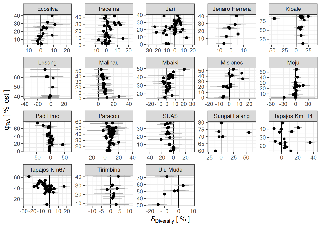
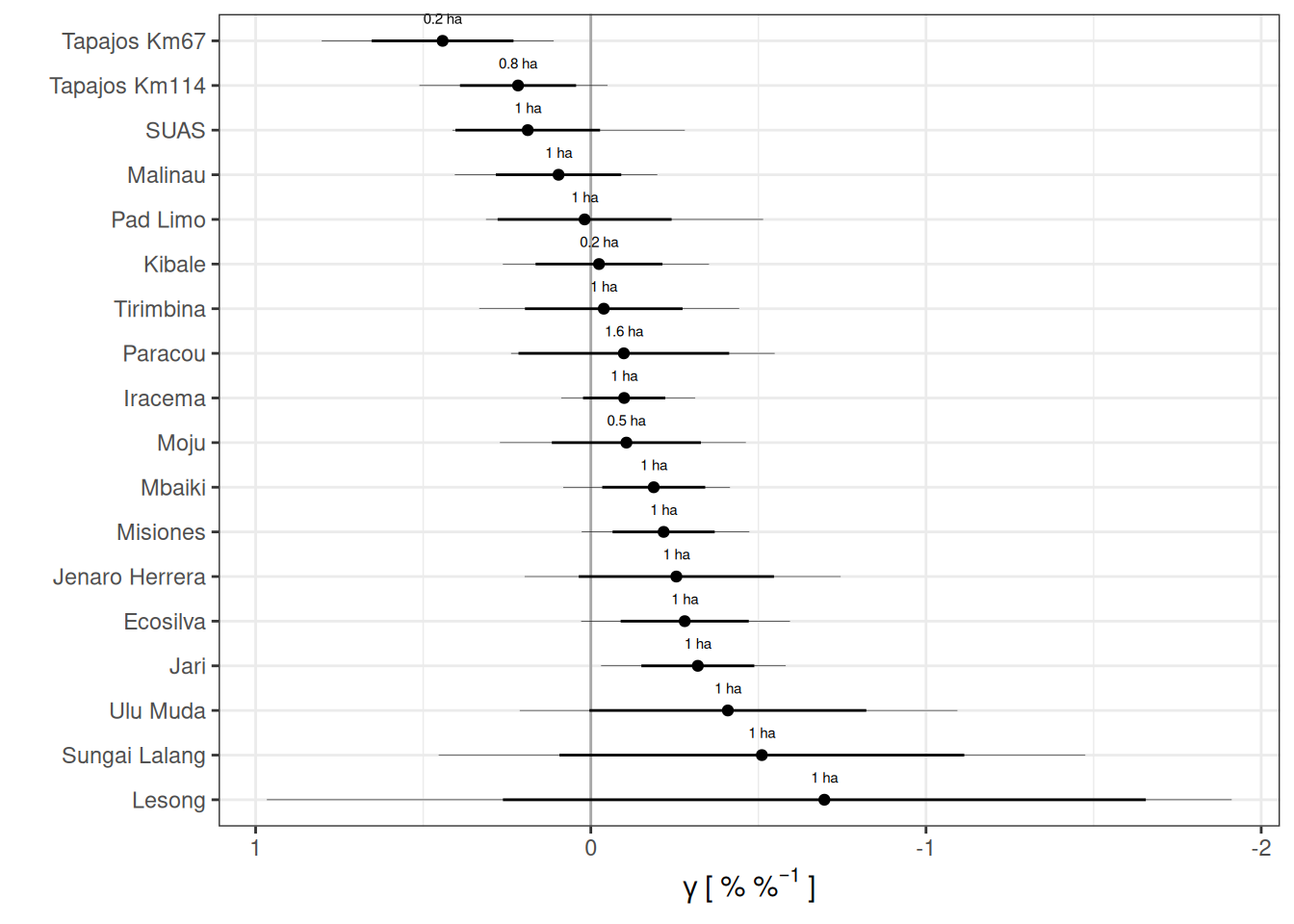
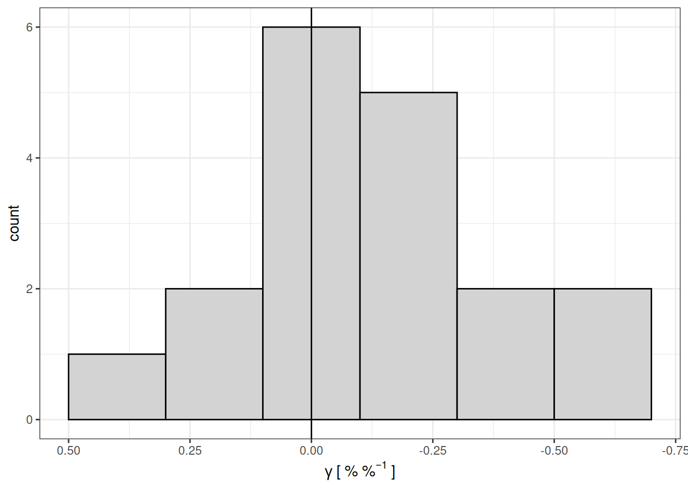
Posteriors of the parameter gamma representing basal are disturbance intensity effect on genus diversity short term increase with plot areas in label.

Code

knitr::include_graphics("chains/gamma_save.png")

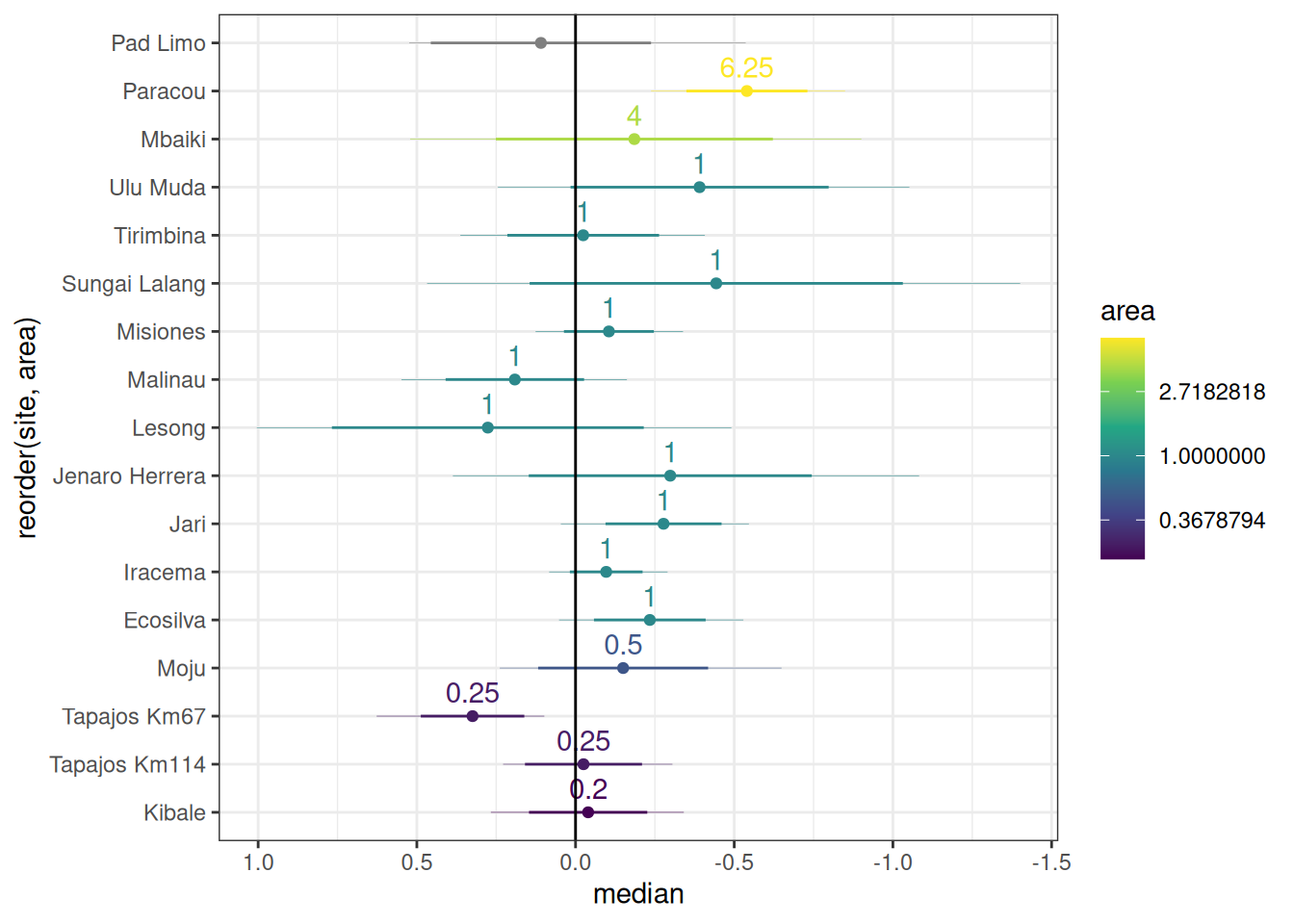
Previous posteriors of the parameter gamma representing basal are disturbance intensity effect on genus diversity short term increase with plot areas in label.

Code

pars_s <- filter(parameters, variable == "gamma") %>% 
  mutate(delta0 = filter(parameters, variable == "delta0")$median)
filter(parameters, variable %in% c("delta", "phiba")) %>% 
  select(site, plot, variable, median) %>% 
  pivot_wider(names_from = variable, values_from = median) %>% 
  ggplot(aes((1-phiba), delta)) +
  facet_wrap(~ site) +
  geom_abline(aes(slope = -mean, 
                  intercept = mean+delta0, group = site), 
              data = pars_s) +
  geom_abline(aes(slope = -mean-sd, 
                  intercept = mean-sd+delta0, group = site), 
              data = pars_s, linetype = "dashed") +
  geom_abline(aes(slope = -mean+sd, 
                  intercept = mean+sd+delta0, group = site), 
              data = pars_s, linetype = "dashed") +
  geom_point() +
  theme_bw() +
  xlab(expression(phi[BA] ~ "[ % lost ]")) +
  ylab(expression(delta[Diversity] ~ "[ % ]")) +
  theme(panel.spacing = unit(0, "lines")) +
  scale_x_continuous(labels = ~.*100) +
  scale_y_continuous(labels = ~.*100)

Inferred relationship between disturbance intensity and diversity short term increase.

Code

filter(parameters, variable == "gamma") %>% 
  ggplot(aes(median)) +
  geom_histogram(fill = "lightgrey", col = "black", binwidth = 0.2) +
  geom_vline(xintercept = 0) +
  theme_bw() +
  scale_x_reverse(expression(gamma~"["~"%"~"%"^{-1}~"]"))

Posteriors of the parameter gamma representing basal are disturbance intensity effect on genus diversity short term increas across sites.